Data cleaning with messy data

ID 529: Data Management and Analytic Workflows in R

Jarvis Chen

Wednesday, January 10, 2024

Follow along

https://bit.ly/messyDataR

Options:
- Download the messy_data.csv file and the id529-day3-messyData.R script
- Or clone the repository and follow along

Learning objectives

In this activity, we’ll look at how to accomplish some common data cleaning tasks using tools from dplyr and the tidyverse
Gain familiarity with the following
- janitor::clean_names() for tidying variable names
- case_when() for recoding variables in mutate()
- across() for mutating multiple columns
- Dealing with duplicates, missingness, and other data messiness
- cut(), quantile(), and dplyr::ntile() for creating categorical variables from continuous variables
- group_by() and summarize() for creating grouped summaries

Messy Data

Read our messy data

For this activity, we created a fake messy dataset with many of the data cleaning tasks that we typically need to accomplish. The data is available on our website as messy_data.csv.

Weird Barbie Our Patron Saint of Messy Data

# Read the messy data
messy_data <- read_csv("messy_data.csv")

# Have a look
View(messy_data)

What do we see?

glimpse(messy_data)

Rows: 182
Columns: 8
$ `ID Number`                     <dbl> 78, 25, 10, 38, 38, 29, 13, 49, 57, 33…
$ `Race self-identified`          <chr> "Black", "White", "Black", "White", "W…
$ `Hispanic ethnicity`            <chr> "Non-Hispanic", "Hispanic", "Non-Hispa…
$ `Age at exam`                   <dbl> 42, 33, 31, -99, 32, 52, -99, 26, -99,…
$ `Self-identified gender`        <chr> "cisgender male", "cisgender male", "c…
$ `Highest education completed`   <chr> "College Grad", "College Grad", "8th G…
$ `Hours of sleep per night`      <dbl> 3.497926, 7.273746, 6.887221, -77.0000…
$ `Household income before taxes` <dbl> 116548.65, 116148.33, 25281.35, -999.0…

The column names have spaces and a mix of capital and lower case letters.
When column names have spaces, we will need to refer to them in quotes, e.g. 'ID Number' – this is very inconvenient!

First, let’s fix the variable names

In general, we would like for there not to be spaces in column names
It is a matter of style, but generally I like to keep things in lower case letters
The janitor::clean_names() function can correct the column names for us!

names(messy_data)

[1] "ID Number"                     "Race self-identified"         
[3] "Hispanic ethnicity"            "Age at exam"                  
[5] "Self-identified gender"        "Highest education completed"  
[7] "Hours of sleep per night"      "Household income before taxes"

df <- messy_data |>
  janitor::clean_names()

names(df)

[1] "id_number"                     "race_self_identified"         
[3] "hispanic_ethnicity"            "age_at_exam"                  
[5] "self_identified_gender"        "highest_education_completed"  
[7] "hours_of_sleep_per_night"      "household_income_before_taxes"

Check how many duplicates there are

Next, we can check how many duplicates there are. The id_number variable identifies subjects, and here we see that some id_number’s appear up to 5 times!

table(df$id_number)


  1   2   3   4   5   6   7   8   9  10  11  12  13  14  15  16  17  18  19  20 
  1   3   1   3   1   1   2   1   2   2   1   2   4   1   1   2   1   1   3   1 
 21  22  23  24  25  26  27  28  29  30  31  32  33  34  35  36  37  38  39  40 
  2   2   1   2   1   1   2   1   1   1   1   2   3   2   2   1   1   5   1   3 
 41  42  43  44  45  46  47  48  49  50  51  52  53  54  55  56  57  58  59  60 
  4   2   3   2   4   2   2   2   1   4   1   1   1   2   3   1   2   4   1   3 
 61  62  63  64  65  66  67  68  69  70  71  72  73  74  75  76  77  78  79  80 
  1   4   1   1   1   1   5   1   1   1   2   1   1   1   1   1   1   1   4   4 
 81  82  83  84  85  86  87  88  89  90  91  92  93  94  95  96  97  98  99 100 
  1   2   1   3   3   2   2   1   3   1   1   1   1   1   2   1   4   1   1   2

Is there a pattern to the duplicated records?

df <- df |> arrange(id_number)
View(df)

In this particular case, it looks like the duplicated records are missing many of the variables.

What’s up with the missing codes?

table(df$self_identified_gender)


         cisgender female            cisgender male non-binary or genderqueer 
                       42                        46                         6 
       transgender female          transgender male                   unknown 
                        1                         5                        82

table(df$hispanic_ethnicity)


    Hispanic Non-Hispanic      unknown 
          35           65           82

table(df$highest_education_completed)


   8th Grade 9-11th Grade College Grad  High School Some College      unknown 
           6           17           29           11           37           82

summary(df$age_at_exam)

   Min. 1st Qu.  Median    Mean 3rd Qu.    Max. 
  -99.0   -99.0    28.0   -22.4    40.0    70.0

summary(df$hours_of_sleep_per_night)

   Min. 1st Qu.  Median    Mean 3rd Qu.    Max. 
-77.000 -77.000   5.022 -30.882   7.245  10.083

summary(df$household_income_before_taxes)

   Min. 1st Qu.  Median    Mean 3rd Qu.    Max. 
   -999    -999   17988   34999   53474  453841

What’s up with the missing codes?

There appear to be various kinds of missingness coded (e.g. “unknown”, -99, -77, and -999), but if we want R to handle them as missing data, we should recode them to NA
We could recode each of these variables one at a time using mutate()

# for example
df |>
  mutate(hispanic_ethnicity = ifelse(hispanic_ethnicity == "unknown",
                                     NA_character_,
                                     hispanic_ethnicity)) |>
  select(hispanic_ethnicity) |>
  unique()

# A tibble: 3 × 1
  hispanic_ethnicity
  <chr>             
1 Non-Hispanic      
2 <NA>              
3 Hispanic

This could get a bit tedious if we have a lot of variables to recode!

Let’s recode the missing values

We can use mutate(across()) to recode these variables more efficiently
across() allows us to apply the same function or a set of functions to multiple columns of a dataframe at once
- this simplifies the code and improves readability
The basic syntax is

mutate(data, across(columns, functions))

columns specifies the columns of the dataframe to apply the function to. This can be a selection of columns like c(col1, col2)
Or we can specify columns using a helper like everything(), starts_with(), ends_with(), contains()

Let’s recode the missing values

df <- df |>
  mutate(across(c(hispanic_ethnicity, self_identified_gender, highest_education_completed),
                ~ ifelse(.x == "unknown", NA_character_, .x)),
         across(c(age_at_exam, hours_of_sleep_per_night, household_income_before_taxes),
                ~ ifelse(.x < 0, NA_real_, .x)))

head(df)

# A tibble: 6 × 8
  id_number race_self_identified             hispanic_ethnicity age_at_exam
      <dbl> <chr>                            <chr>                    <dbl>
1         1 American Indian or Alaska Native Non-Hispanic                51
2         2 White                            <NA>                        NA
3         2 White                            <NA>                        NA
4         2 White                            Non-Hispanic                55
5         3 Two or more races                Non-Hispanic                35
6         4 Black                            <NA>                        NA
# ℹ 4 more variables: self_identified_gender <chr>,
#   highest_education_completed <chr>, hours_of_sleep_per_night <dbl>,
#   household_income_before_taxes <dbl>

Now we can deal with the duplicates!

We can count up how many missing variables there are for each of the multiple records and use this information to help us select the duplicated record with the most complete data (discarding the other incomplete records).

# count the number of missing columns
df$missing_count = rowSums(is.na(df), na.rm = FALSE)

# create a new dataframe with unique id's
unique_df <- df |>
  # group by id_number
  group_by(id_number) |>
  # sort each id_number's observations by the number of missing columns (from fewest to most)
  arrange(missing_count) |>
  # take the first row for each id_number, which is the row with the fewest missing variables
  slice(1) |>
  # drop the missing_count variable
  select(-missing_count) |>
  # it's always a good idea to ungroup() after using a group_by
  ungroup()

View(unique_df)

Collapsing categories

For some variables, we often need to collapse categories to ensure enough subjects for analysis.

table(unique_df$race_self_identified, unique_df$hispanic_ethnicity)

                                     
                                      Hispanic Non-Hispanic
  American Indian or Alaska Native           0            4
  Asian                                      8            8
  Black                                      8           16
  Native Hawaiian or Pacific Islander        0            4
  Two or more races                          1            1
  White                                     18           32

table(unique_df$self_identified_gender)


         cisgender female            cisgender male non-binary or genderqueer 
                       42                        46                         6 
       transgender female          transgender male 
                        1                         5

table(unique_df$highest_education_completed)


   8th Grade 9-11th Grade College Grad  High School Some College 
           6           17           29           11           37

Collapsing categories

The dplyr::case_when() function is a versatile tool for recoding variables. When used with dplyr::mutate, it allows you to transform a variable’s values based on a set of conditions, making it especially useful in data manipulation and cleaning.
The basic syntax is:

df <- df |>
  mutate(new_var = case_when(
      condition1 ~ value1, 
      condition2 ~ value2, 
      ...,
      TRUE ~ default_value))

Collapsing racial/ethnic groups

Here, we create a collapsed racial/ethnic variable called raceth that combines information from race_self_identified and hispanic_ethnicity
We’ll combine subjects who are Non-Hispanic American Indian or Alaskan Native, Non-Hispanic Asian or Pacific Islander, and Non-Hispanic Two or more races into a category we’ll call “underrepresented racial/ethnic group”

unique_df <- unique_df |>
  mutate(raceth = factor(
    case_when(
      race_self_identified == "White" &
        hispanic_ethnicity == "Non-Hispanic" ~ "Non-Hispanic White",
      race_self_identified == "Black" &
        hispanic_ethnicity == "Non-Hispanic" ~ "Non-Hispanic Black",
      hispanic_ethnicity == "Hispanic" ~ "Hispanic",
      is.na(race_self_identified) |
        is.na(hispanic_ethnicity) ~ NA_character_,
      TRUE ~ "underrepresented racial/ethnic group"
    ),
    levels = c(
      "Non-Hispanic White",
      "Non-Hispanic Black",
      "Hispanic",
      "underrepresented racial/ethnic group"
    )
  ))

Collapsing racial/ethnic groups

table(unique_df$raceth)


                  Non-Hispanic White                   Non-Hispanic Black 
                                  32                                   16 
                            Hispanic underrepresented racial/ethnic group 
                                  35                                   17

Collapsing gender and education

We can similarly recode gender and education into collapsed categories

unique_df <- unique_df |>
  mutate(
    gender_collapsed = ifelse(
      self_identified_gender %in% c(
        "transgender female",
        "transgender male",
        "non-binary or genderqueer"
      ),
      "trans/non-binary",
      self_identified_gender
    ),
    education_collapsed = case_when(
      highest_education_completed %in% c("8th Grade", "9-11th Grade") ~ "less than hs",
      highest_education_completed %in% c("High School", "Some College") ~ "hs grad",
      highest_education_completed == "College Grad" ~ "college grad"
    )
  )

Note the use of ifelse(test, yes, no) where test is a logical vector (condition to be tested), yes is a value to return if test is TRUE, and no is a value to return if test is FALSE

Collapsing gender and education

table(unique_df$gender_collapsed)


cisgender female   cisgender male trans/non-binary 
              42               46               12

table(unique_df$education_collapsed)


college grad      hs grad less than hs 
          29           48           23

Categorizing continuous variables

Now suppose that we want to create a dichotomous variable for insufficient_sleep based on hours_of_sleep_per_night (<7 hours per night is insufficient sleep)

unique_df <- unique_df |>
  mutate(insufficient_sleep = hours_of_sleep_per_night < 7)

table(unique_df$insufficient_sleep)


FALSE  TRUE 
   52    48

Categorizing continuous variables

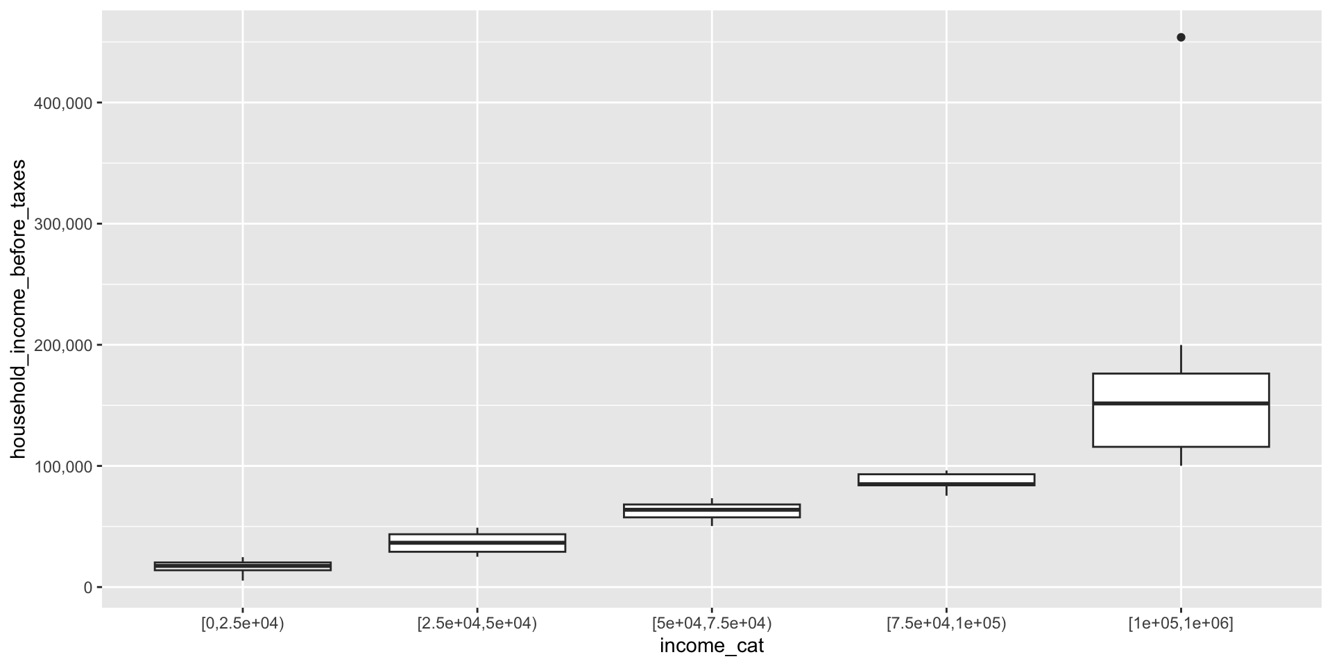
We can use the cut() function to create categories from a continuous variable (here, household_income_before_taxes) by supplying a list of cutpoints (breaks)
dplyr has a function ntile() that creates approximately equal sized groups (e.g. quintiles)

unique_df <- unique_df |>
  mutate(income_cat = cut(household_income_before_taxes, 
                          breaks = c(0, 25000, 50000, 75000, 100000, 1000000),
                          right = FALSE, include.lowest=TRUE, na.rm=T),
         income_quint = ntile(household_income_before_taxes, 5))

Categories using cut()

ggplot(unique_df, 
       aes(x=income_cat, y=household_income_before_taxes)) + 
  geom_boxplot() +
  scale_y_continuous(labels=label_comma())

Categories using ntile()

ggplot(unique_df, 
       aes(x=factor(income_quint), y=household_income_before_taxes)) + 
  geom_boxplot()

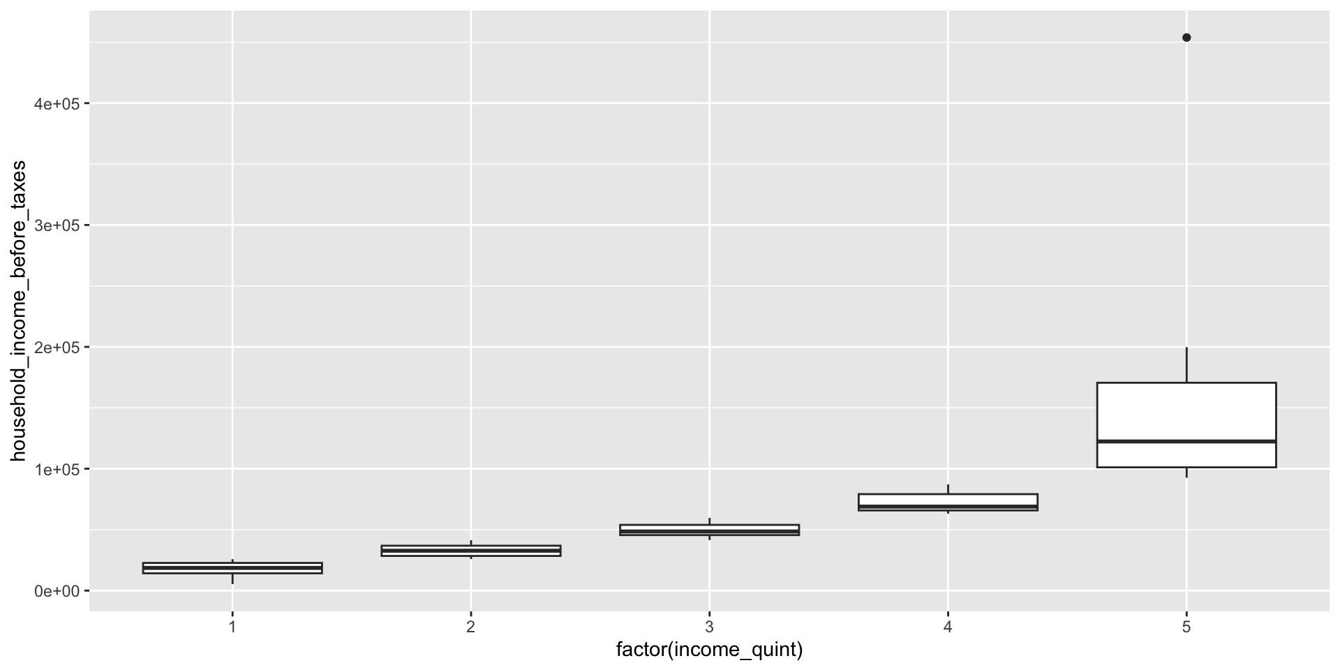
Note that ntile() has recoded household_income_before_taxes into categories directly, but we don’t know what the cutpoints are

Using group_by() and summarize()

We can use group_by() and summarize() to get information about the range of values in each category of income_quint

unique_df |>
  group_by(income_quint) |>
  summarise(mininc = min(household_income_before_taxes, na.rm=T),
            maxinc = max(household_income_before_taxes, na.rm=T))

# A tibble: 5 × 3
  income_quint mininc  maxinc
         <int>  <dbl>   <dbl>
1            1  5355.  25771.
2            2 25884.  41372.
3            3 41393.  59690.
4            4 63073.  87118.
5            5 92593. 453841.

group_by() and summarize()

group_by()
- group_by() is used to split a data frame into groups based on one or more variables. This function doesn’t change the data itself but changes its metadata, setting up for grouped operations like summarizing or mutating each group separately.
summarize()
- summarize() – or summarise() – is used to collapse each group created by group_by() into a single-row summary based on specified summary functions.
- While group_by() doesn’t change the data, summarize() does

group_by() and summarize()

Some commonly used functions in summarize() are:
- mean(): Calculates the mean (average) of a numeric column.
- sum(): Computes the sum of a numeric column.
- min() and max(): Find the minimum or maximum value of a column.
- n(): Counts the number of observations in a group.
- n_distinct(): Counts the number of unique values in a column.
- median(): Finds the median of a numeric column.
- sd(): Computes the standard deviation of a numeric column.

Example: calculating proportions

Suppose we want to calculate the proportion of subjects in each gender and racial/ethnic group who have sufficient and insufficient sleep

proportions_by_gender_raceth <- unique_df |>
  group_by(gender_collapsed, raceth, insufficient_sleep) |>
  summarize(count_insufficient_sleep = n(), .groups='drop') |>
  group_by(gender_collapsed, raceth) |>
  mutate(proportion_insufficient_sleep = 
           count_insufficient_sleep/sum(count_insufficient_sleep, na.rm=T)) |>
  ungroup()

View(proportions_by_gender_raceth)

Note the use of .groups='drop' in the summarize statement. This says to remove the grouping after summarizing (equivalent to ungroup())

Example: calculating mean, median, and sd

With summarize, we can use across to create multiple summary columns

summarize_continuous_variables <- unique_df |>
  summarize(across(
    c(
      age_at_exam,
      hours_of_sleep_per_night,
      household_income_before_taxes
    ),
    list(
      mean = ~ mean(.x, , na.rm = TRUE),
      median = ~ median(.x, na.rm = TRUE),
      sd = ~ sd(.x, na.rm = TRUE)
    )
  ))

View(summarize_continuous_variables)

Note that
- we supplied a list of functions for summarize to apply to each column specified
- summarize automatically created names for the new columns in the summary dataframe
- .x is explicitly used as a placeholder to refer to an element being acted upon (here, each of the columns specified in the call to across)