Diverse Data Sources
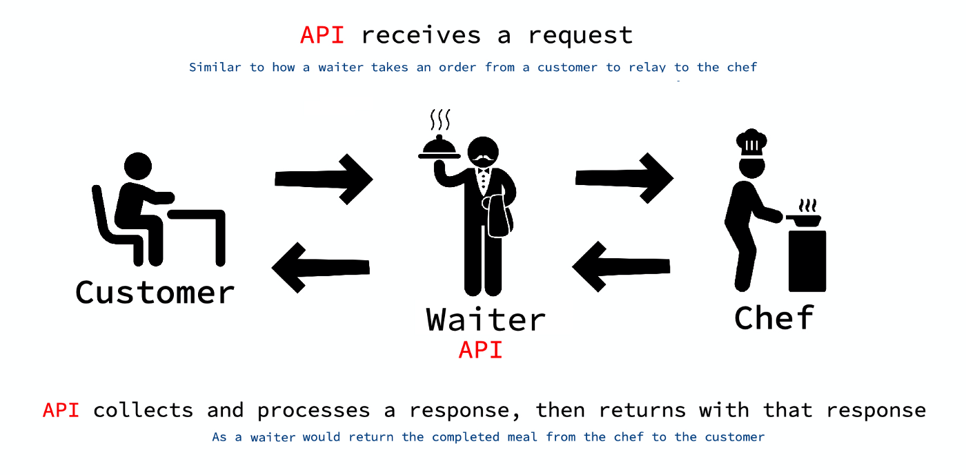
moral

not all data will be handed to you in a tabular form

some alternative data sources

  • application programming interfaces (APIs)
  • the content on websites
  • PDF documents
  • images of text/tables

APIs

what is an API?

a good analogy for an API is the wait-staff
at a restaurant:  the wait-staff collect the order from the customer, deliver
that to the back of the house, and then once the food is ready, deliver that
to the customer.

common APIs

some common examples of APIs include services like websites, apps like Uber/Lyft, Google Maps, etc. – all of these operate on the principle that you structure your request and their server will send back the response.

some examples in plain language:

  • request: “give me the URL at https://google.com”

  • response: “sure, here are the files (some HTML, CSS, and JS)”

  • request: “I need a ride to ____”

  • response: “we can book you a ride for $XX” (probably in JSON sent to your app)

the way you’re most likely used to interfacing with these APIs is through an app (like a web browser or native app on your phone), but it’s also completely possible to send and receive your API requests in code.

working with APIs

you can use the httr and httr packages in R if you need to work directly with APIs. these are built on the curl commandline utility.

however, there’s a good chance you won’t need to work with httr or httr2 because many popular APIs have “wrappers” already written in R that make working with them much simpler.

a note on secrets

if you are using an API where you must authenticate your account DO NOT put your credentials or private keys/tokens into anything publicly shared including git version tracked files that leave your computer, files on GitHub, or Google Docs or anywhere else online.

why? because API keys are valuable to nefarious actors and people scrape GitHub and other public sites to find API keys that they can abuse.

a note on secrets

here’s a disaster scenario: let’s say you sign up for an Amazon Web Services account with a credit card, and connect to their API in your code so you can automatically spin-up new virtualized servers as you need them, but your API key gets shared on GitHub.

someone could find that and use that to pay for their crazy computing endeavors (mining Bitcoin, illegal stuff, whatever), and then you could be stuck with an insane $$$$ credit card bill.

handling secrets

if you work with API keys/tokens/authentication that should be kept secret, store them in one of the following:

  • files stored outside your project (ideally encrypted at rest)
  • use something like the secret or secure package to store your secrets encrypted and keep the encryption passphrase/key out of your version control software.

one option that works that I don’t recommend is using .gitignore to ensure that the files with the secrets don’t end up on GitHub – it’s very easy to accidentally screw up and it can be a challenge to get your API keys off git/GitHub (read: re-writing history on git is a bit tricky).

some API wrappers you might enjoy

tidycensus

tidycensus is an R package that allows users to interface with a select number of the US Census Bureau’s data APIs and return tidyverse-ready data frames, optionally with simple feature geometry included.

install.packages("tidycensus")

library(tidycensus)
library(tidyverse)

census_api_key("YOUR API KEY GOES HERE")

county_poverty <- tidycensus::get_acs(
  geography = 'county',
  year = 2020,
  variables = 
    c(people_in_poverty = 'B05010_002',
      total_in_poverty_table = 'B05010_001'),
  geometry = TRUE)

tidycensus

tidycensus

with a little bit more code, you can produce from those data something like this:
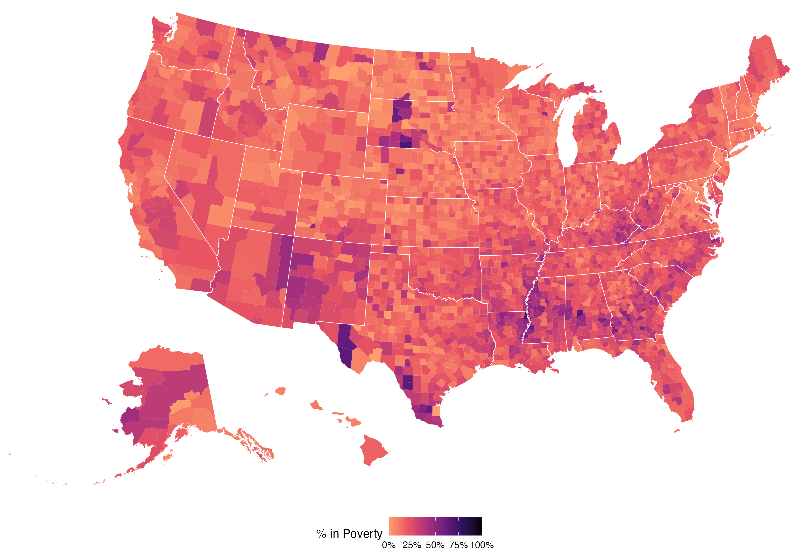
a map of poverty rates by US county

tidycensus

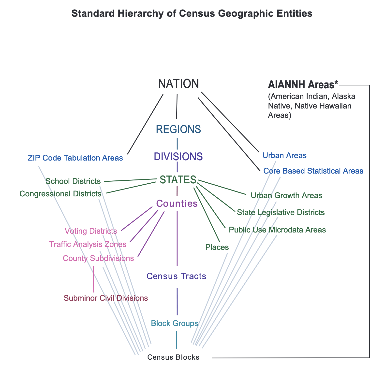
tidycensus is an incredibly useful resource if you’re doing population health research in the United States setting because the Census provides data through several survey based products at a wide range of geographic levels on a huge number of topics.

the geographic hierarchy of the Census: along the main spine
are census blocks, block groups, census tracts, counties, states, divisions, regions, and the nation; 
off of the main spine there are other things like subminor civil divisions, statistical areas, zip codes, school districts, american indian alaska native areas, etc.

word cloud of subjects covered in the census

qualtRics

Qualtrics is an online survey and data collection software platform. Qualtrics is used across many domains in both academia and industry for online surveys and research. While users can manually download survey responses from Qualtrics through a browser, importing this data into R is then cumbersome.

https://docs.ropensci.org/qualtRics/

qualtRics

install.packages("qualtRics")
library(qualtRics)

# get setup - only run once
qualtrics_api_credentials(api_key = "<YOUR-QUALTRICS_API_KEY>", 
                          base_url = "<YOUR-QUALTRICS_BASE_URL>",
                          install = TRUE)
                          
# fetch your surveys
surveys <- all_surveys() 

# get a specific survey 
mysurvey <- fetch_survey(surveyID = surveys$id[6], 
                         verbose = TRUE)
                         
head(mysurvey)
# A tibble: 143 × 449
# … with 449 variables: StartDate <chr>, EndDate <chr>, Status <chr>, IPAddress <chr>, Progress <chr>,
#   Duration (in seconds) <chr>, Finished <chr>, RecordedDate <chr>, ResponseId <chr>,
#   RecipientLastName <chr>, RecipientFirstName <chr>, RecipientEmail <chr>, ExternalReference <chr>,
#   LocationLatitude <chr>, LocationLongitude <chr>, DistributionChannel <chr>, UserLanguage <chr>, …
# ℹ Use `colnames()` to see all variable names

a few APIs just to mention

World Bank

https://data.worldbank.org/ provides a ton of global development indicators data across countries. there are two packages out that provide user-friendly interfaces in R: WDI and wbstats.

the World Health Organization Global Health Observatory

https://www.who.int/data/gho provides many datasets on health and disease from all over the world.

the WHO (https://github.com/expersso/WHO) package provides a programmatic interface to retrieve data from the WHO Global Health Observatory from entirely within R.

Bureau of Labor Statistics

The US Bureau of Labor Statistics “measures labor market activity, working conditions, price changes, and productivity in the U.S. economy to support public and private decision making.”

They have an API too! https://www.bls.gov/developers/

And there’s an R wrapper for their API as well: https://github.com/mikeasilva/blsAPI

scraping websites

rvest

using the rvest package, you can parse the HTML contents of a web-page into a format you can work with in R.

install.packages(“rvest”)
library(rvest)

literacy <- read_html("https://en.wikipedia.org/wiki/List_of_countries_by_literacy_rate")
html_tables <- literacy |> html_nodes(".wikitable")
html_tables[[1]] |> html_table()

#    Country               `Youth(15 to 24)` `Youth(15 to 24)` Adult(…¹ Adult…² Elder…³ Elder…⁴ Youth…⁵ Youth…⁶
#    <chr>                 <chr>             <chr>             <chr>    <chr>   <chr>   <chr>   <chr>   <chr>  
#  1 Country               "Rate"            "Year"            "Rate"   "Year"  "Rate"  "Year"  "Rate"  "Year" 
#  2 Afghanistan*          "47.0"            "2011"            "31.7"   "2011"  "20.3"  "2011"  "0.5"   "2011" 
#  3 Albania*              "99.2"            "2012"            "97.2"   "2012"  "86.9"  "2012"  "1.0"   "2012" 
#  4 Algeria*              "93.8"            "2008"            "75.1"   "2008"  "19.5"  "2008"  "1.0"   "2008" 
#  5 American Samoa*       "97.7"            "1980"            "97.3"   "1980"  "92.7"  "1980"  "1.0"   "1980" 
#  6 Andorra*              ""                ""                ""       ""      ""      ""      ""      ""     
#  7 Angola*               "77.4"            "2014"            "66.0"   "2014"  "27.0"  "2014"  "0.8"   "2014" 
#  8 Anguilla*             "99.1"            "1984"            "95.4"   "1984"  "88.0"  "1984"  "1.0"   "1984" 
#  9 Antigua and Barbuda*  ""                ""                "98.9"   "2015"  ""      ""      ""      ""     
# 10 Argentina*            "99.5"            "2016"            "99.1"   "2016"  "97.9"  "2016"  "1.0"   "2016" 
# # … with 225 more rows, and abbreviated variable names ¹`Adult(25+)`, ²`Adult(25+)`, ³`Elderly(65+)`,
# #   ⁴`Elderly(65+)`, ⁵`Youth GenderParity Index`, ⁶`Youth GenderParity Index`
# # ℹ Use `print(n = ...)` to see more rows

the polite package

just note that not all websites take kindly to web scraping, and you should be conscientious of this. check websites’ robots.txt file to find out their policy for scraping.

or use the polite package:

# remotes::install_github("dmi3kno/polite")  # to install
library(polite)  # respectful webscraping

# Make our intentions known to the website
reddit_bow <- bow(
  url = "https://www.reddit.com/",  # base URL
  user_agent = "C Testa <https://id529.github.io>",  # identify ourselves
  force = TRUE
)

print(reddit_bow)
# <polite session> https://www.reddit.com/
#     User-agent: C Testa <https://id529.github.io>
#     robots.txt: 45 rules are defined for 7 bots
#    Crawl delay: 5 sec
#   The path is scrapable for this user-agent

getting tables out of pdf documents

sometimes we are in the annoying situation of having to re-digitize data that has been rendered in a pdf document.

in those situations, the tabulizer package may help you out. the syntax is fairly straightforward, but do be warned that automated solutions like these can be prone to typos and formatting glitches.

screen recording of tabulizer package digitizing some pdf tables

extracting text from images

occasionally you may find yourself in the bind of having images that contain text data you’d like to extract. in computer science, this problem is called “optical character recognition” or OCR, and there’s some handy OCR software that has an R interface we can use.
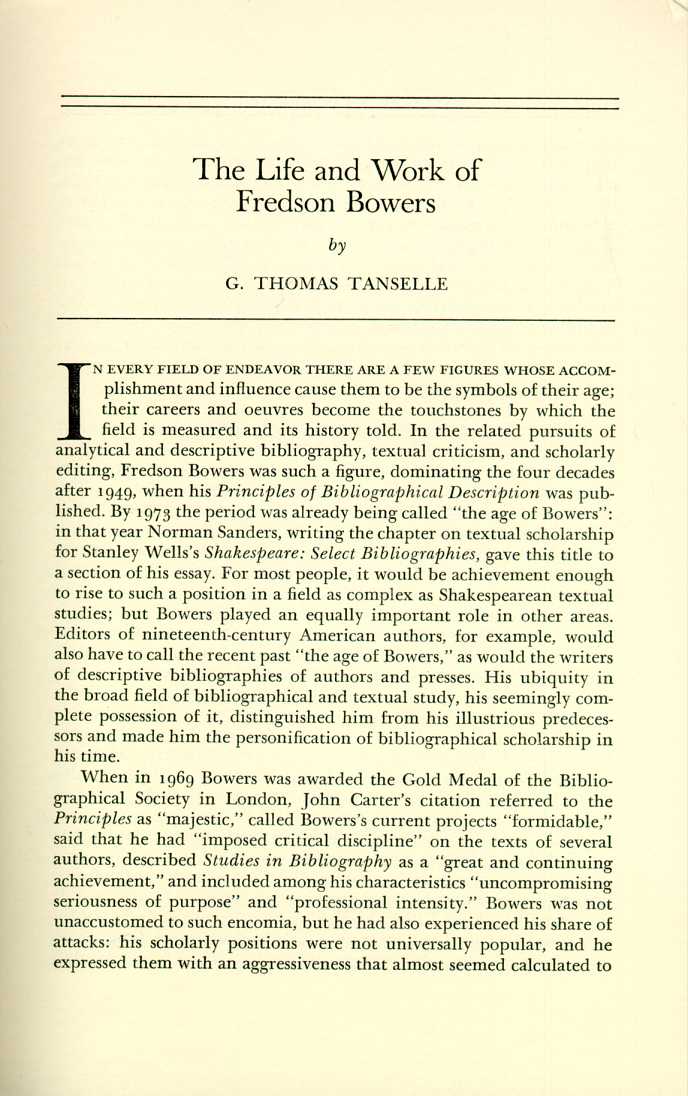
a picture of a book chapter

library(tesseract)
eng <- tesseract("eng")
text <- tesseract::ocr("https://jeroen.github.io/images/bowers.jpg", engine = eng)
cat(text)
# The Life and Work of
# Fredson Bowers
# by
# G. THOMAS TANSELLE
# 
# N EVERY FIELD OF ENDEAVOR THERE ARE A FEW FIGURES WHOSE ACCOM-
# plishment and influence cause them to be the symbols of their age;
# their careers and oeuvres become the touchstones by which the
# field is measured and its history told. In the related pursuits of
# analytical and descriptive bibliography, textual criticism, and scholarly
# editing, Fredson Bowers was such a figure, dominating the four decades
# after 1949, when his Principles of Bibliographical Description was pub-
# lished. By 1973 the period was already being called “the age of Bowers”:
# in that year Norman Sanders, writing the chapter on textual scholarship
# for Stanley Wells's Shakespeare: Select Bibliographies, gave this title to
# a section of his essay. For most people, it would be achievement enough
# to rise to such a position in a field as complex as Shakespearean textual
# studies; but Bowers played an equally important role in other areas.
# Editors of nineteenth-century American authors, for example, would
# also have to call the recent past “the age of Bowers,” as would the writers
# of descriptive bibliographies of authors and presses. His ubiquity in
# the broad field of bibliographical and textual study, his seemingly com-
# plete possession of it, distinguished him from his illustrious predeces-
# sors and made him the personification of bibliographical scholarship in
# 
# his time.
# 
# When in 1969 Bowers was awarded the Gold Medal of the Biblio-
# graphical Society in London, John Carter's citation referred to the
# Principles as “majestic,” called Bowers's current projects “formidable,”
# said that he had “imposed critical discipline” on the texts of several
# authors, described Studies in Bibliography as a “great and continuing
# achievement,” and included among his characteristics “uncompromising
# seriousness of purpose” and “professional intensity.” Bowers was not
# unaccustomed to such encomia, but he had also experienced his share of
# attacks: his scholarly positions were not universally popular, and he
# expressed them with an aggressiveness that almost seemed calculated to

datapasta

lastly, we want to show you the datapasta package which allows you to quickly copy & paste tables into R.

an example
showing the datapasta workflow where you can copy and paste tables from HTML into R using datapasta

datapasta

i would say that you shouldn’t use datapasta as a crutch, but rather that it can facilitate some of your prototyping and exploratory analysis.

takeaways

  • the web is full of data you can make use of
  • APIs and API wrappers in R exist to help you make use of it
  • when the data is in an annoying format like in a PDF or in images, you may well be able to extract it