library(tidyverse)
library(sf)
# you might have some data in a shapefile --
# data/shapefile_unzipped/
# -- cb_2013_us_county_20m.dbf
# -- cb_2013_us_county_20m.prj
# -- cb_2013_us_county_20m.shp
# -- cb_2013_us_county_20m.shp.iso.xml
# -- cb_2013_us_county_20m.shp.xml
# -- cb_2013_us_county_20m.shx
# -- county_20m.ea.iso.xml
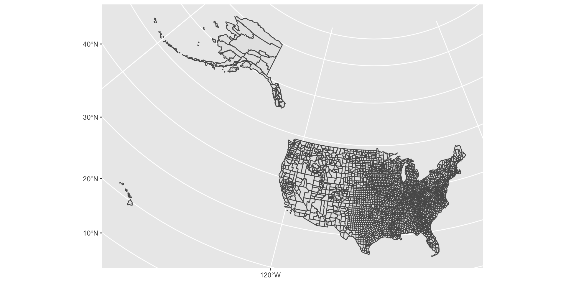
counties <- read_sf(here("data/shapefile_unzipped"))Mapping in R
tigris

tigris is an R package that allows users to directly download and use TIGER/Line shapefiles
sf
the payoff is that then you can use geom_sf() with ggplot2

fixing a problem
or even better
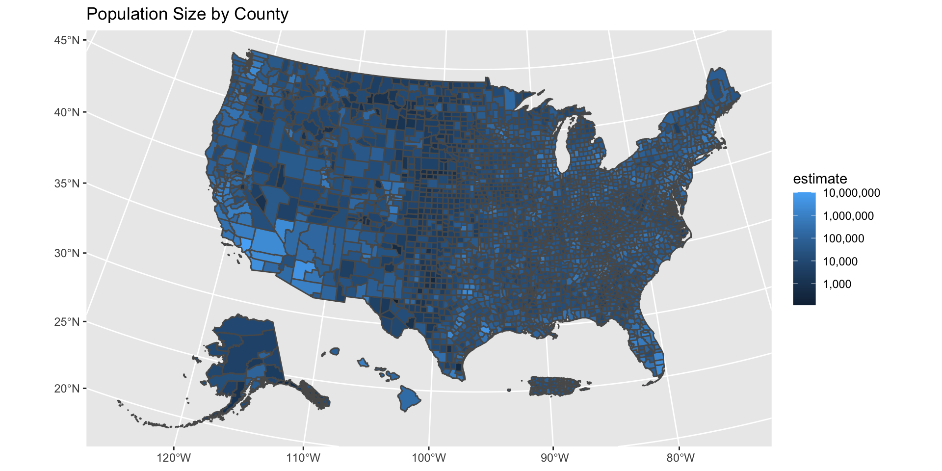
# let's get a more interesting dataset
library(tidycensus)
popsize_by_counties <- tidycensus::get_acs(
year = 2020,
geography = 'county',
variables = "B01001_001", # total population size
geometry = TRUE
)
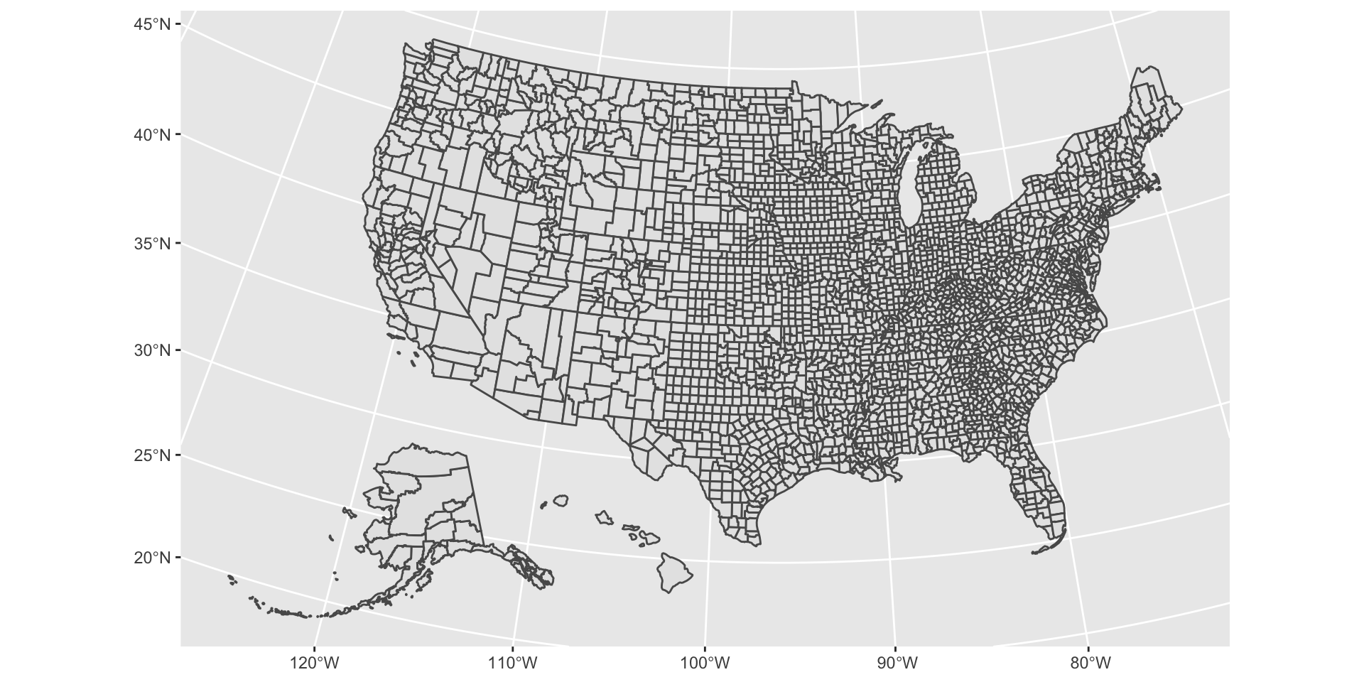
popsize_by_counties <- tigris::shift_geometry(popsize_by_counties)
popsize_by_counties <- st_simplify(popsize_by_counties, dTolerance = 500)
ggplot(popsize_by_counties, aes(fill = estimate)) +
geom_sf()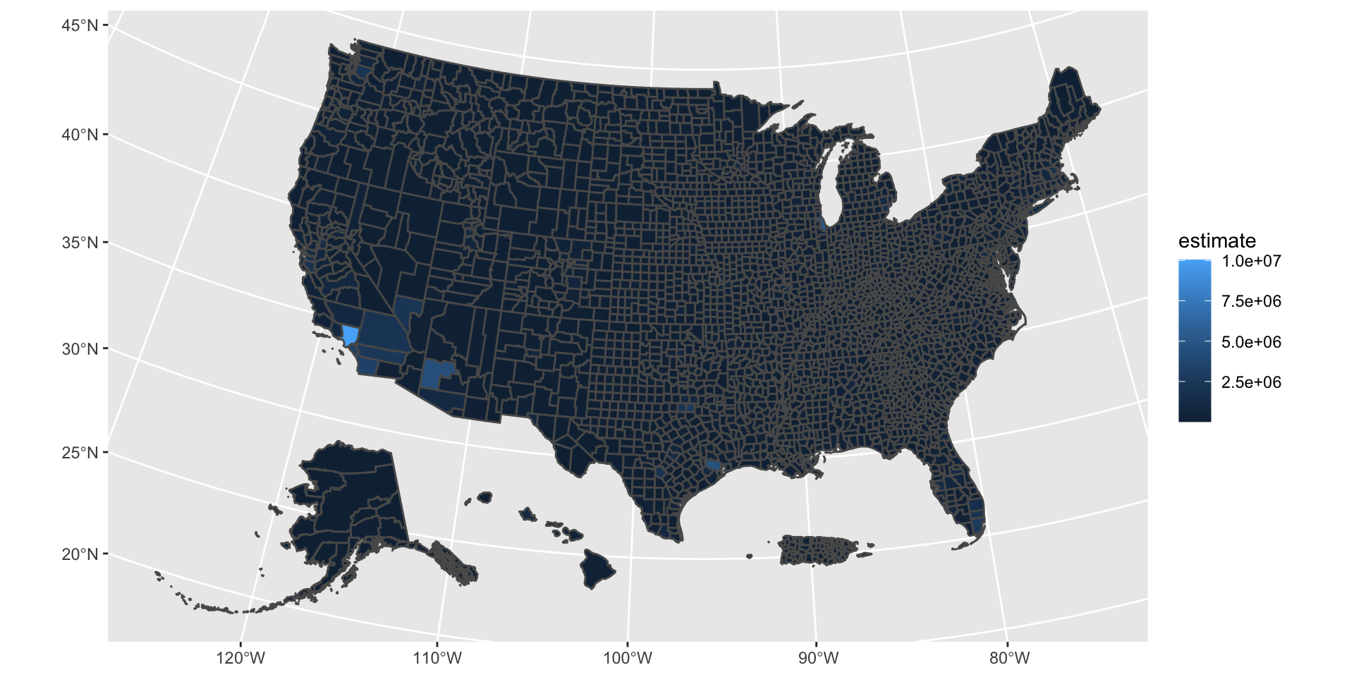
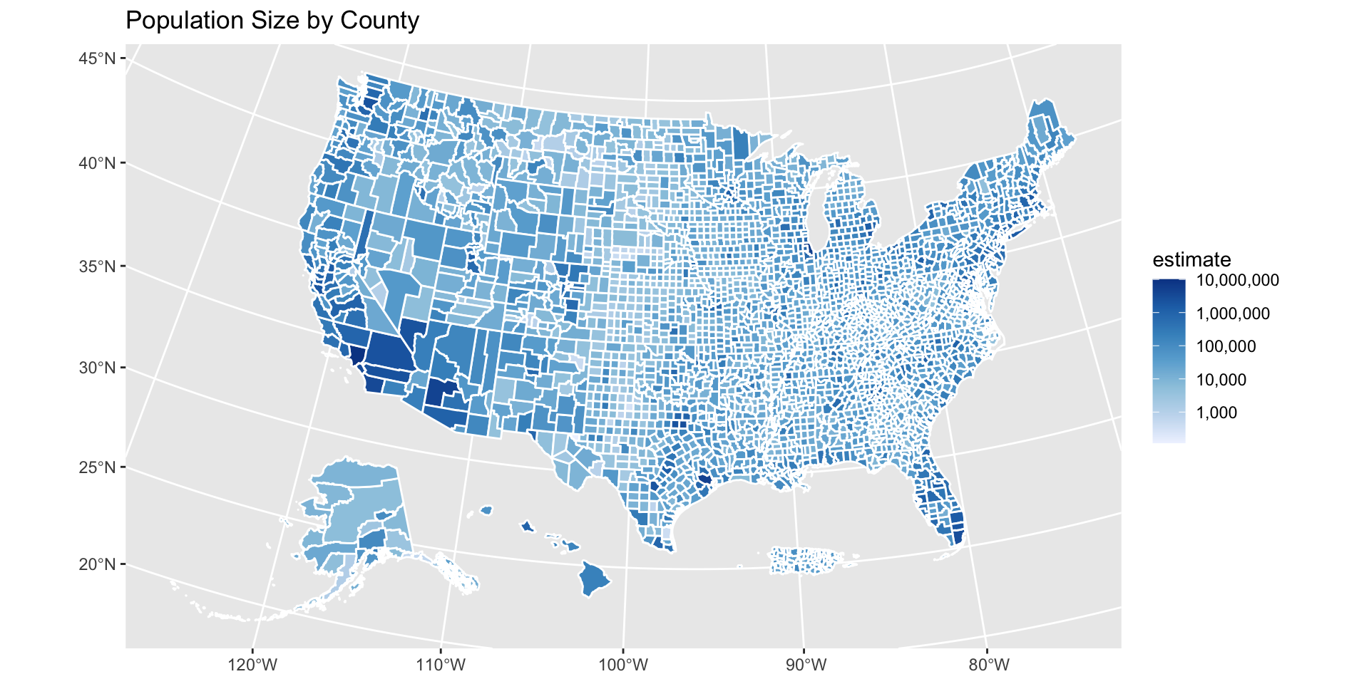
keep improving
keep improving
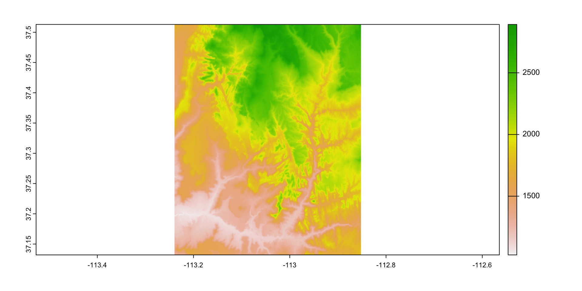
terra
using the terra package, you can work with raster data.