R and RStudio: the basics

installing R and RStudio
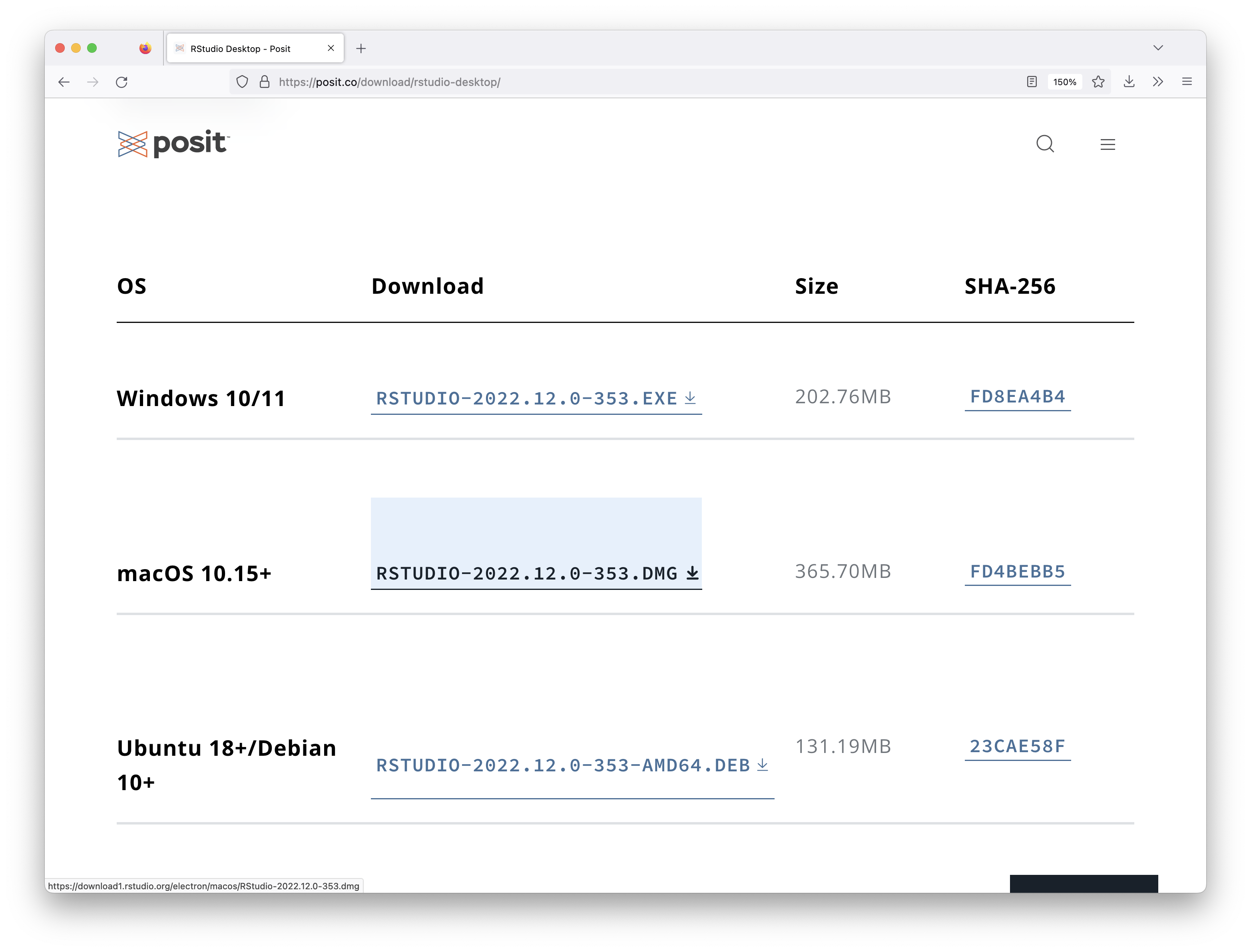
If you haven’t installed R and RStudio yet, please download and install them from here:
installing R and RStudio
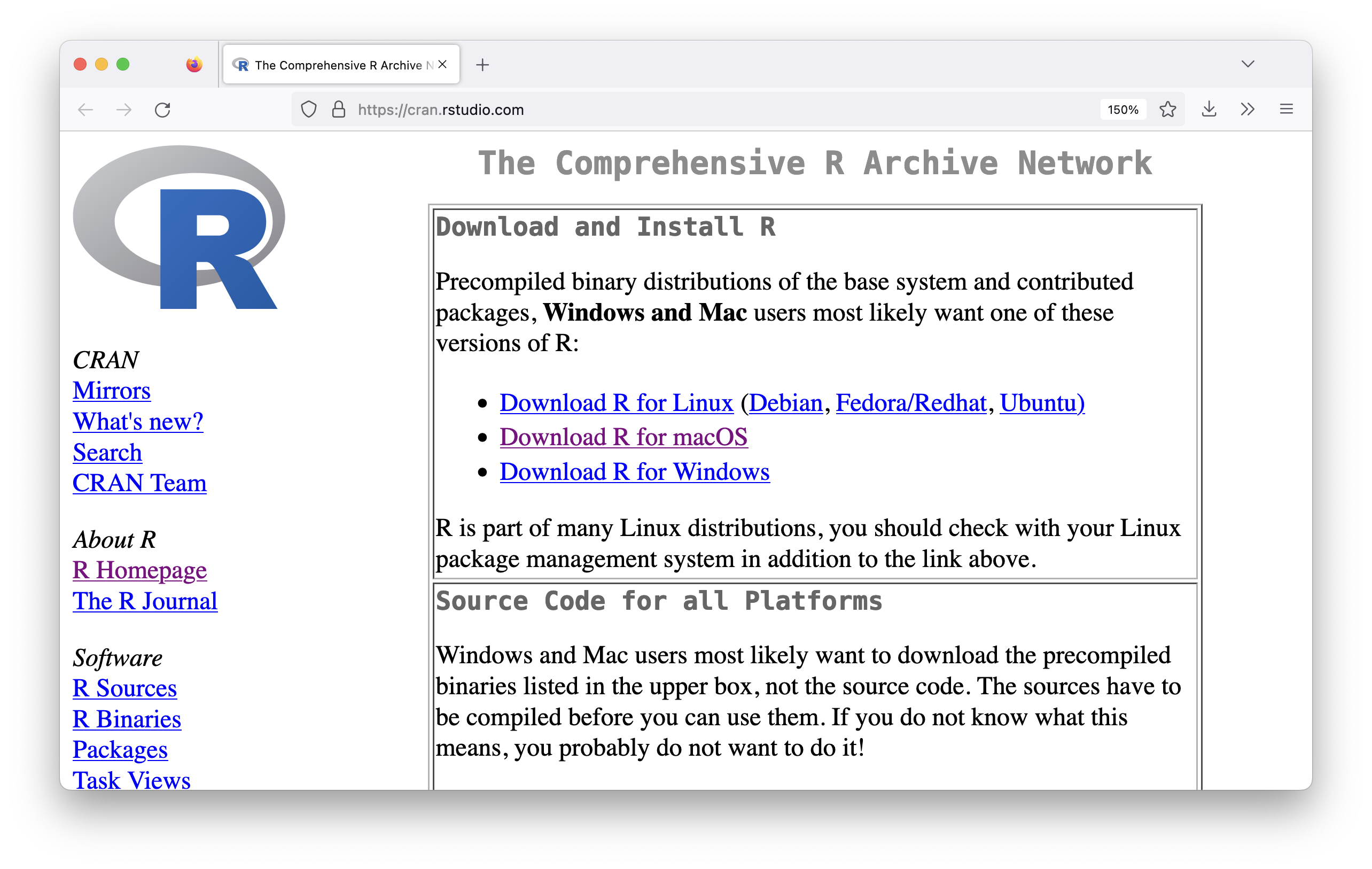
installing R and RStudio

installing R and RStudio
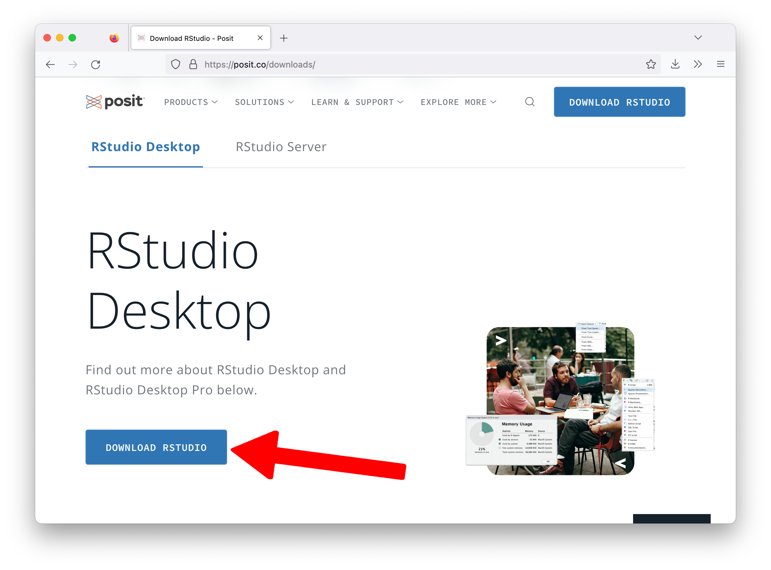
installing R and RStudio
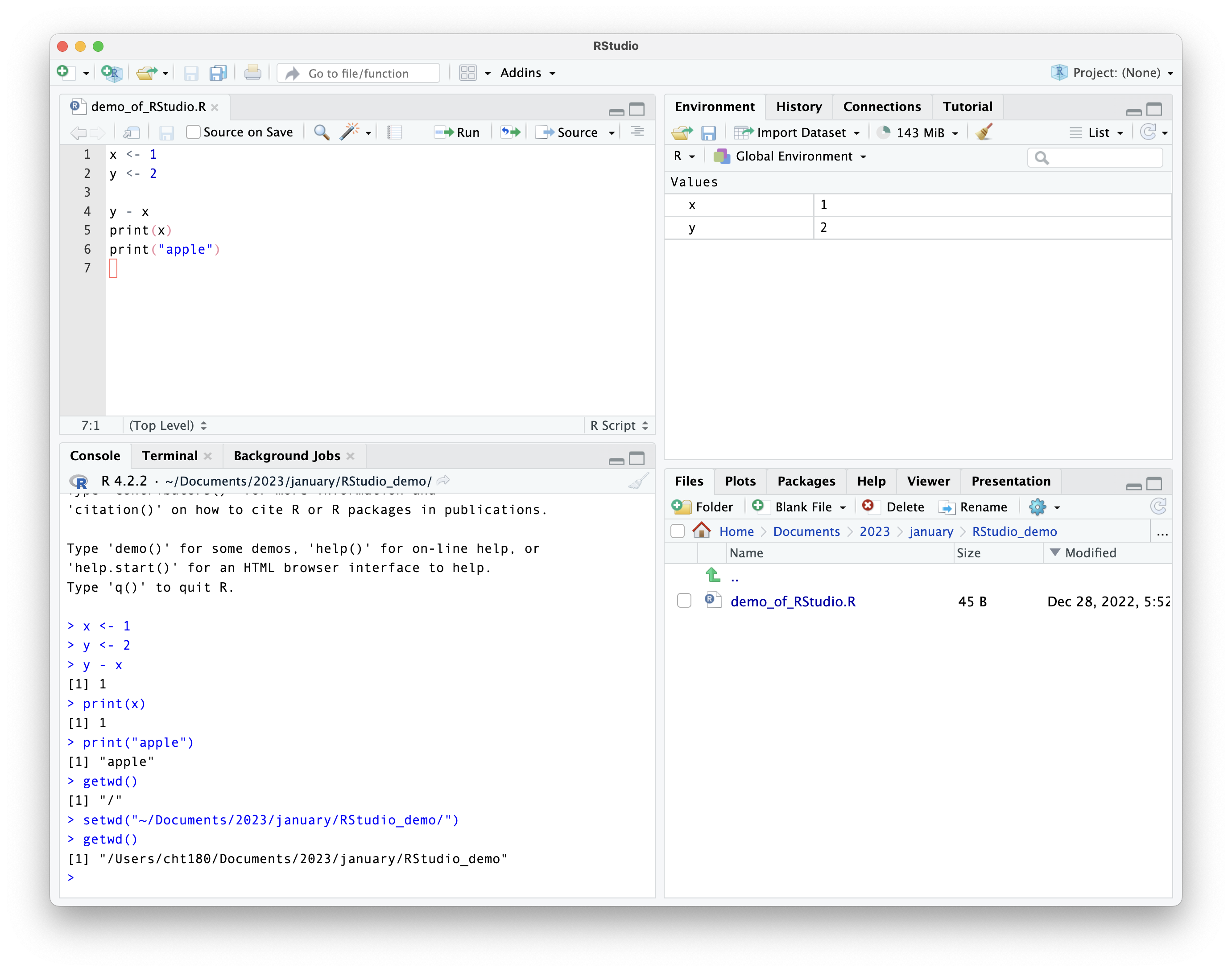
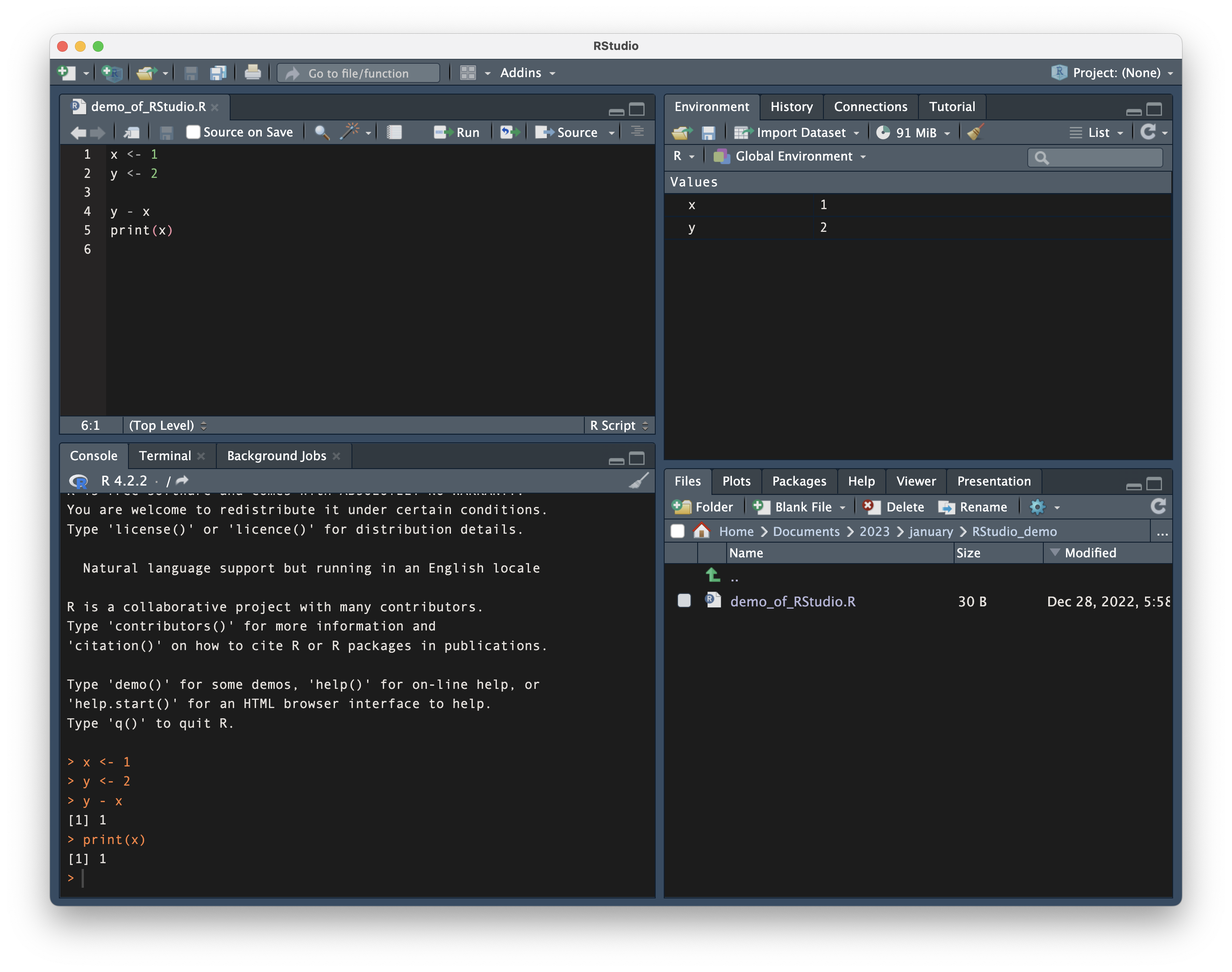
let’s start with RStudio
RStudio
first let’s talk about what the different panes are.
source pane
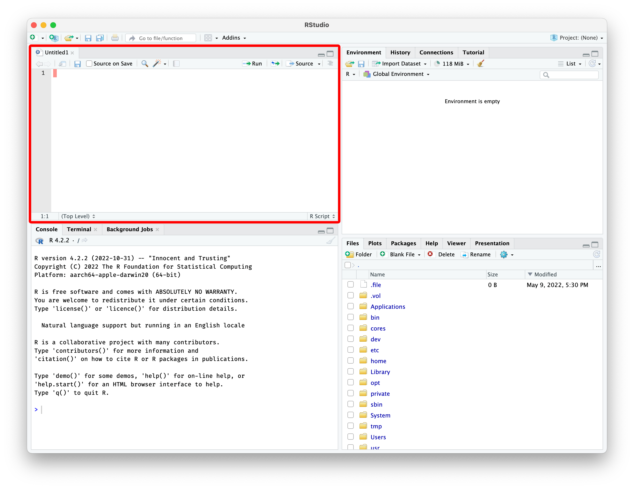
console pane
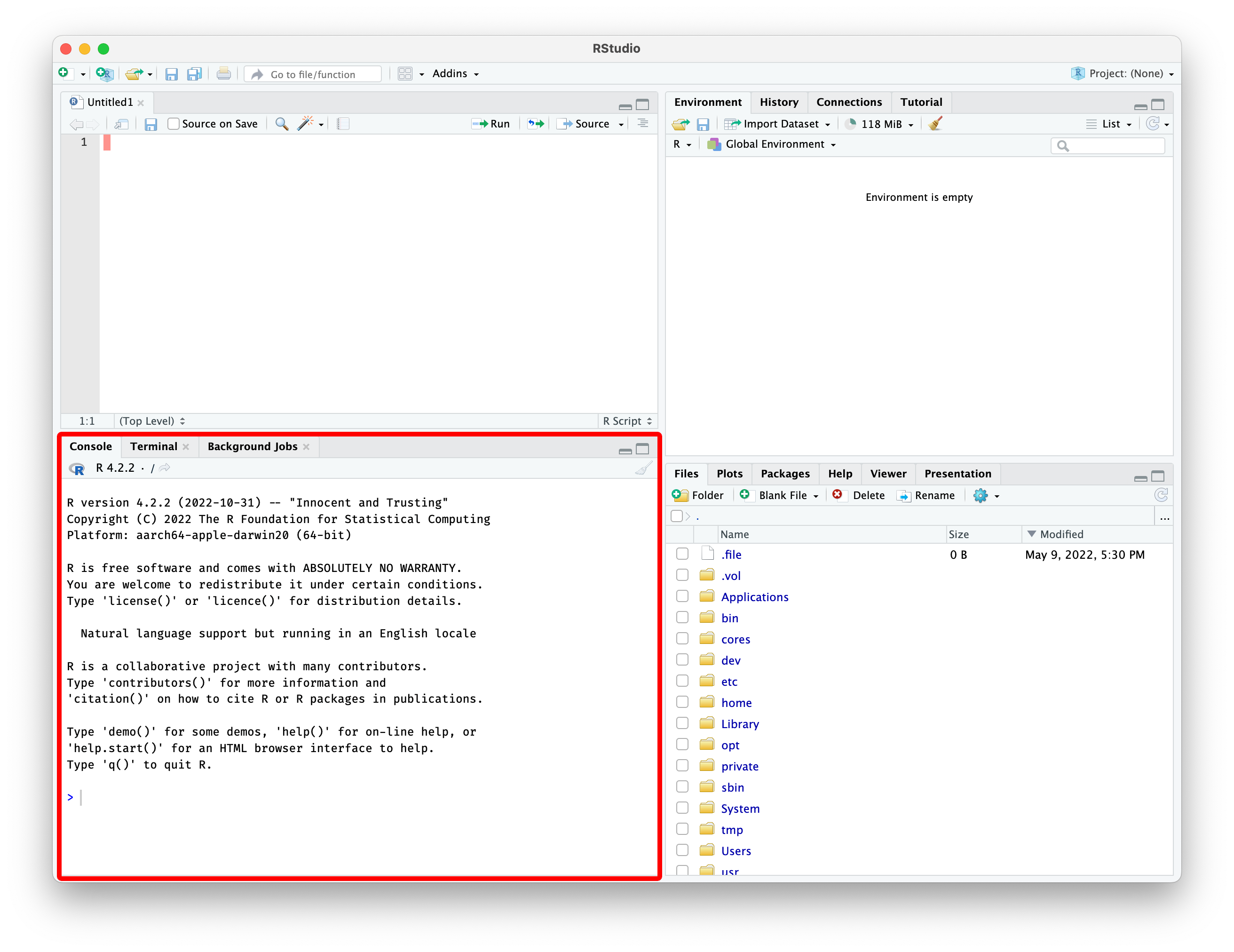
environment pane
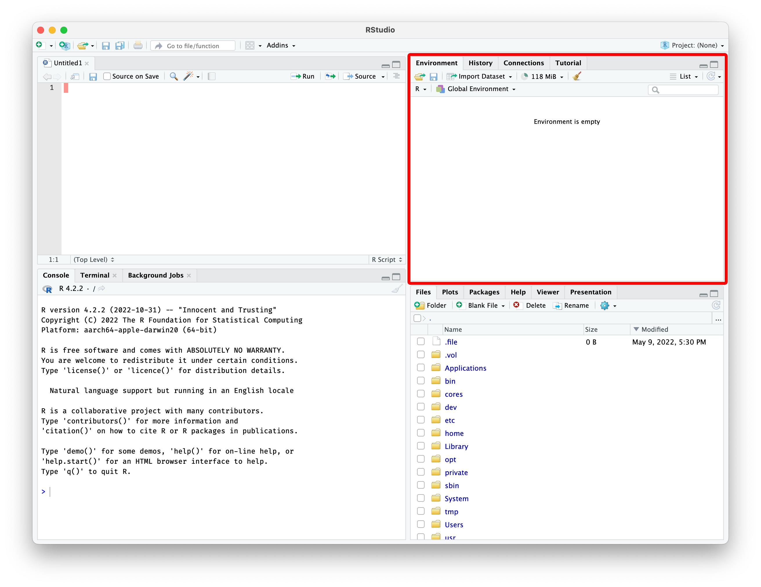
files pane
writing code
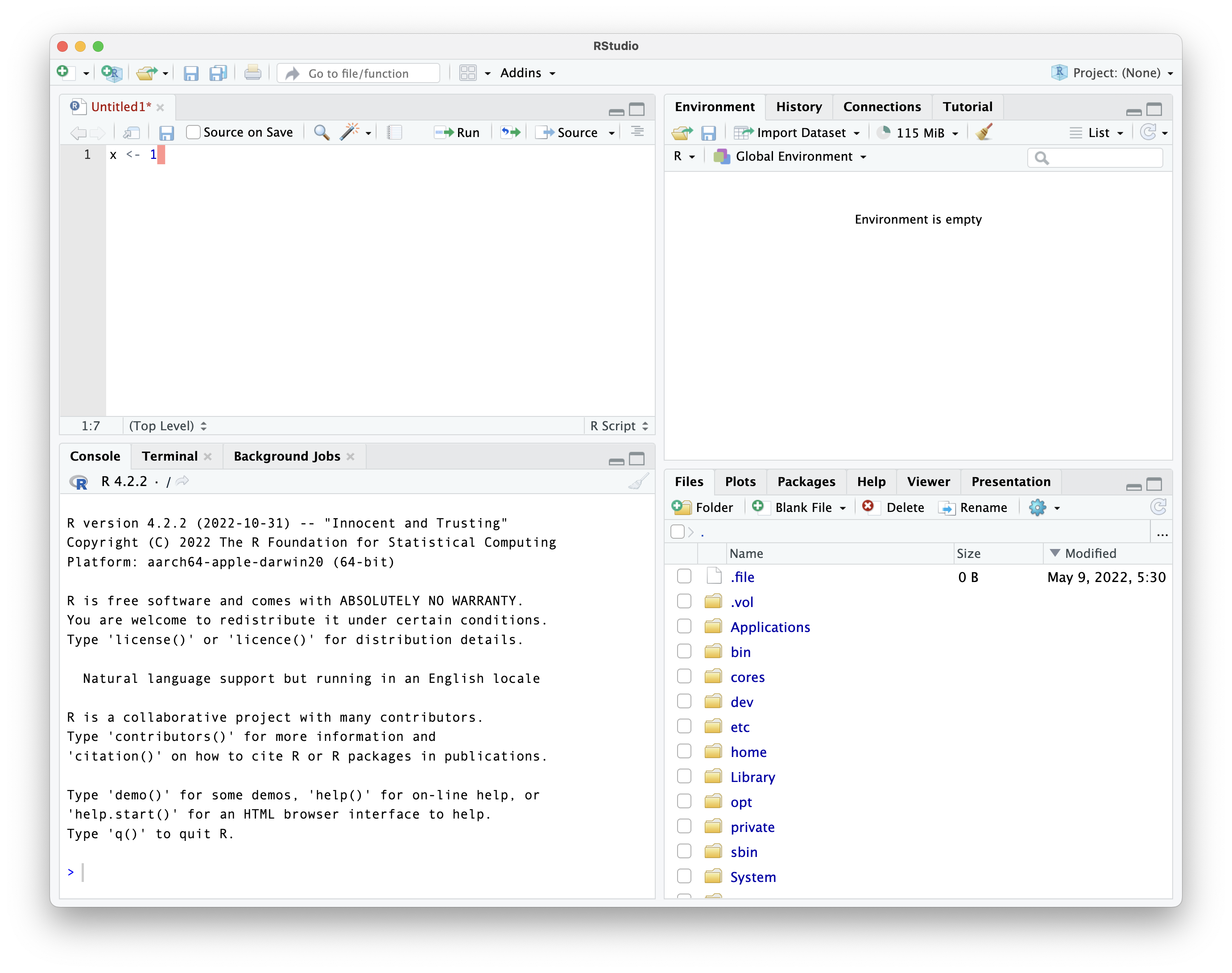
run button
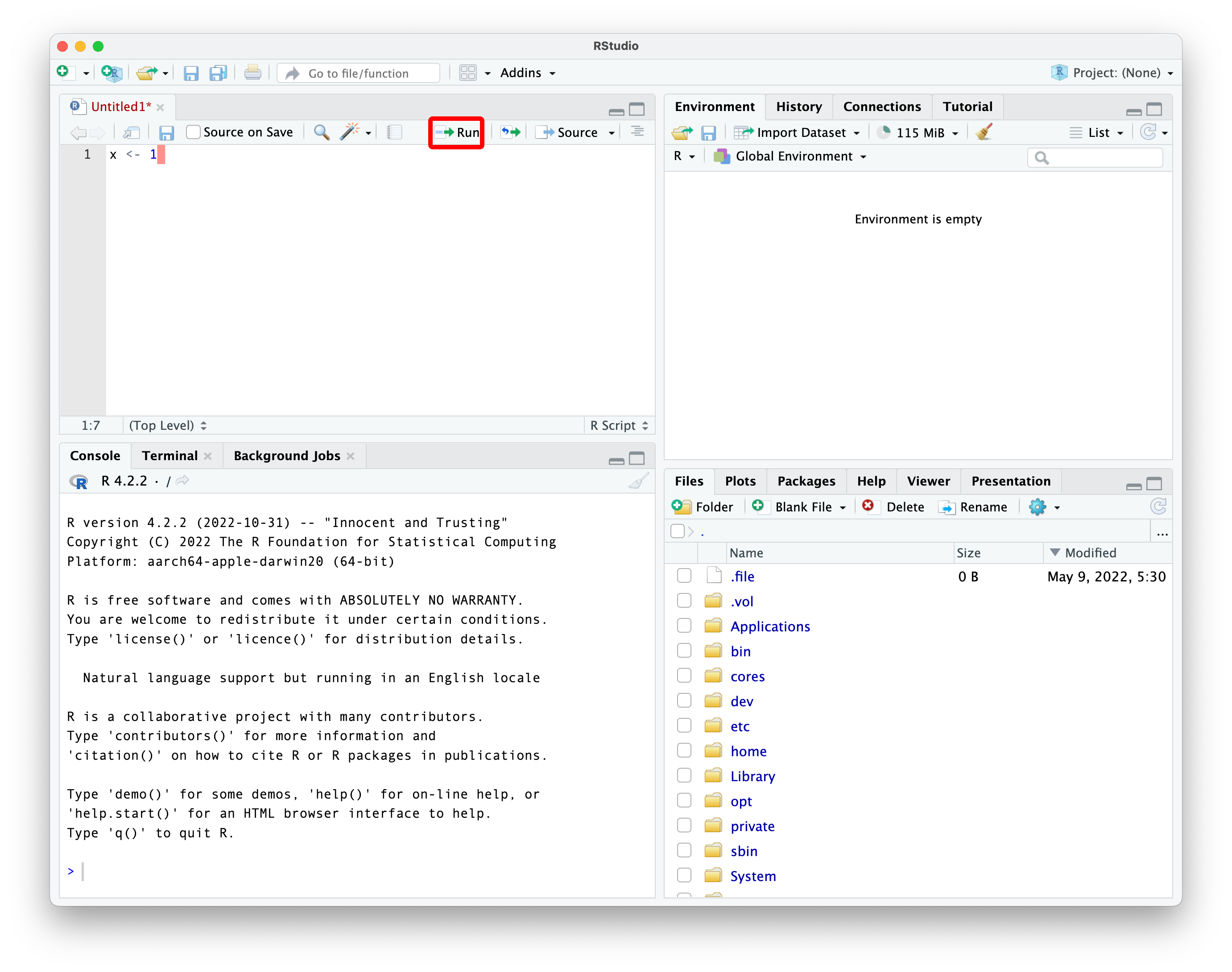
the result of running that line
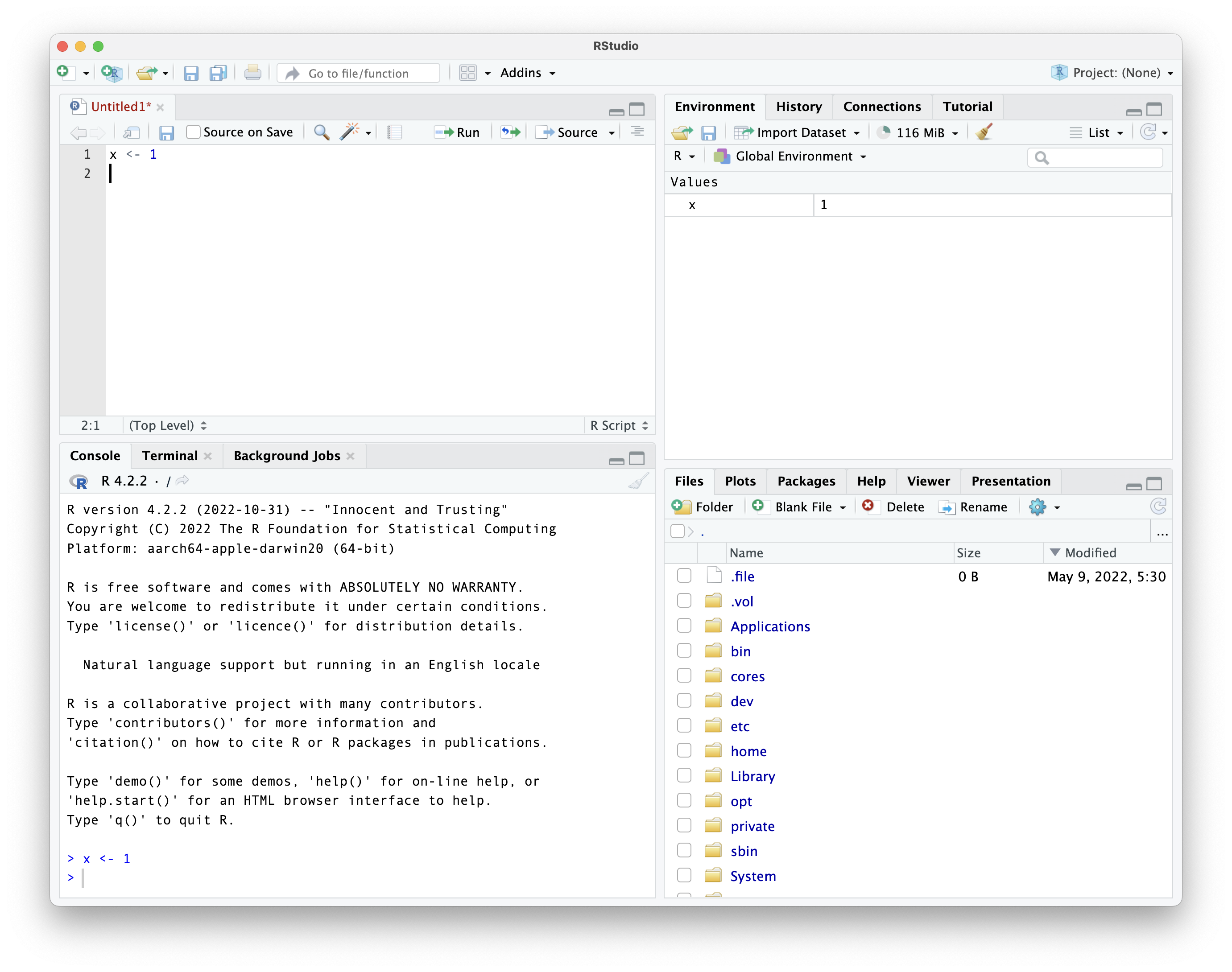
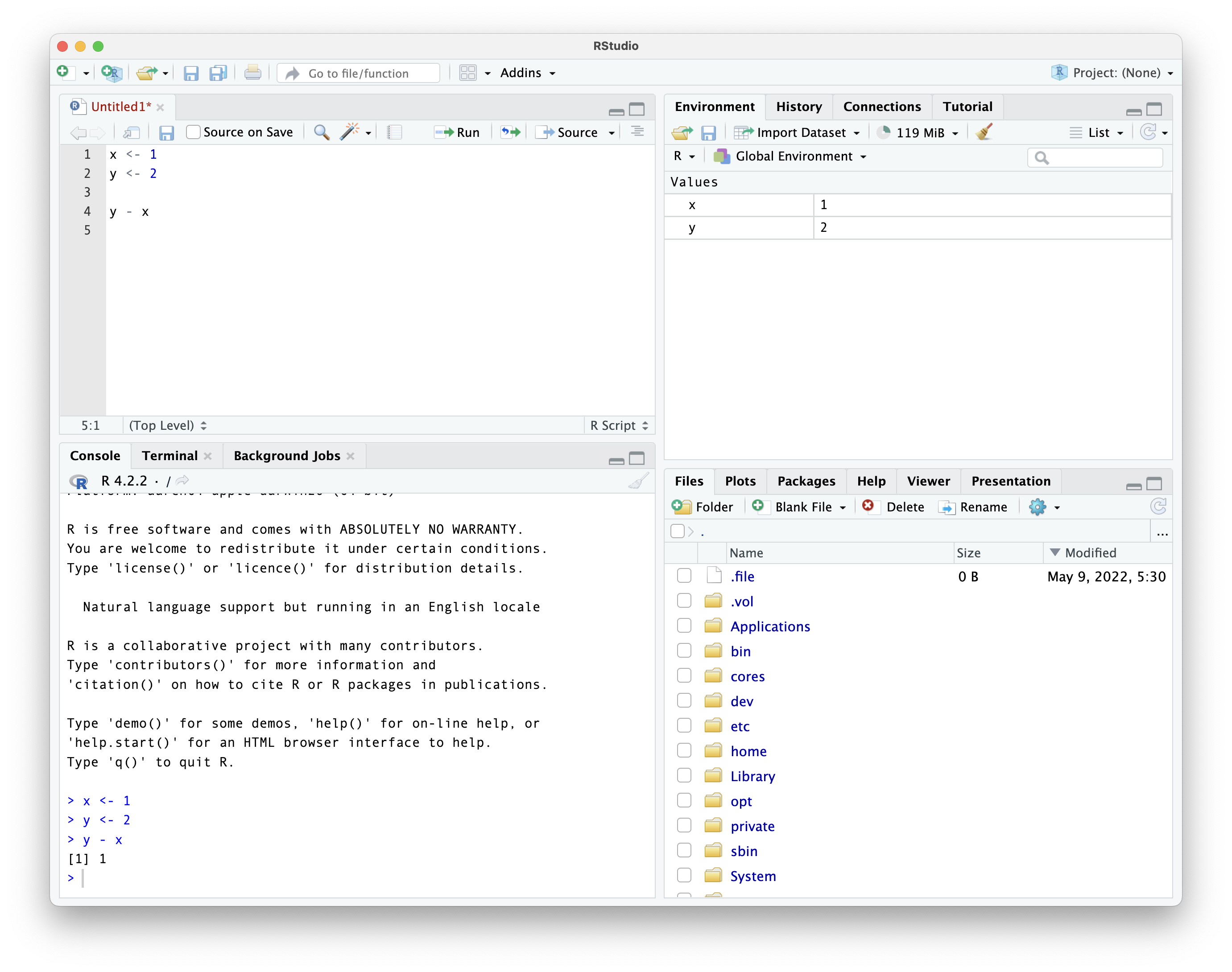
we can run more code
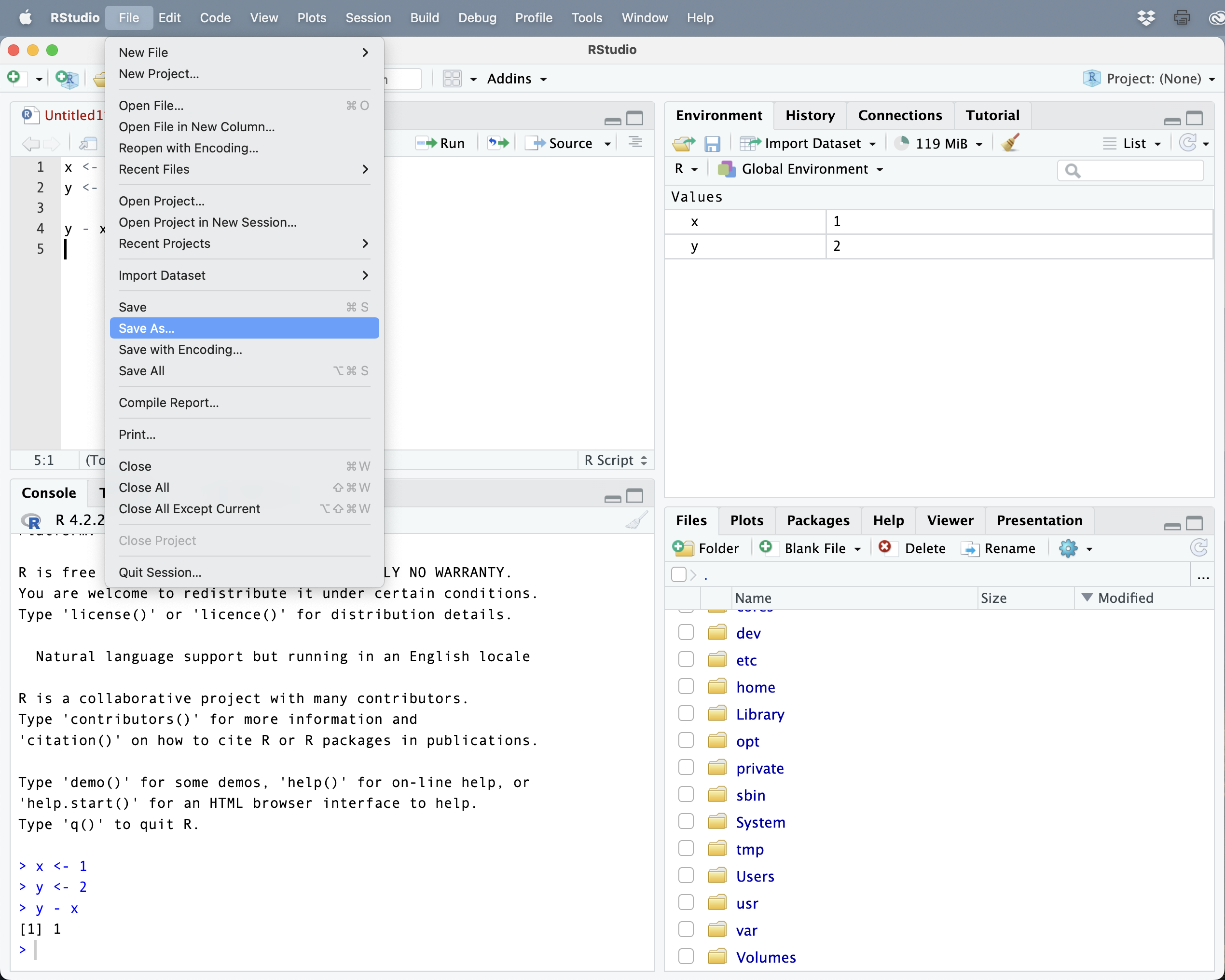
File → Save As
the print command

navigating using the file pane
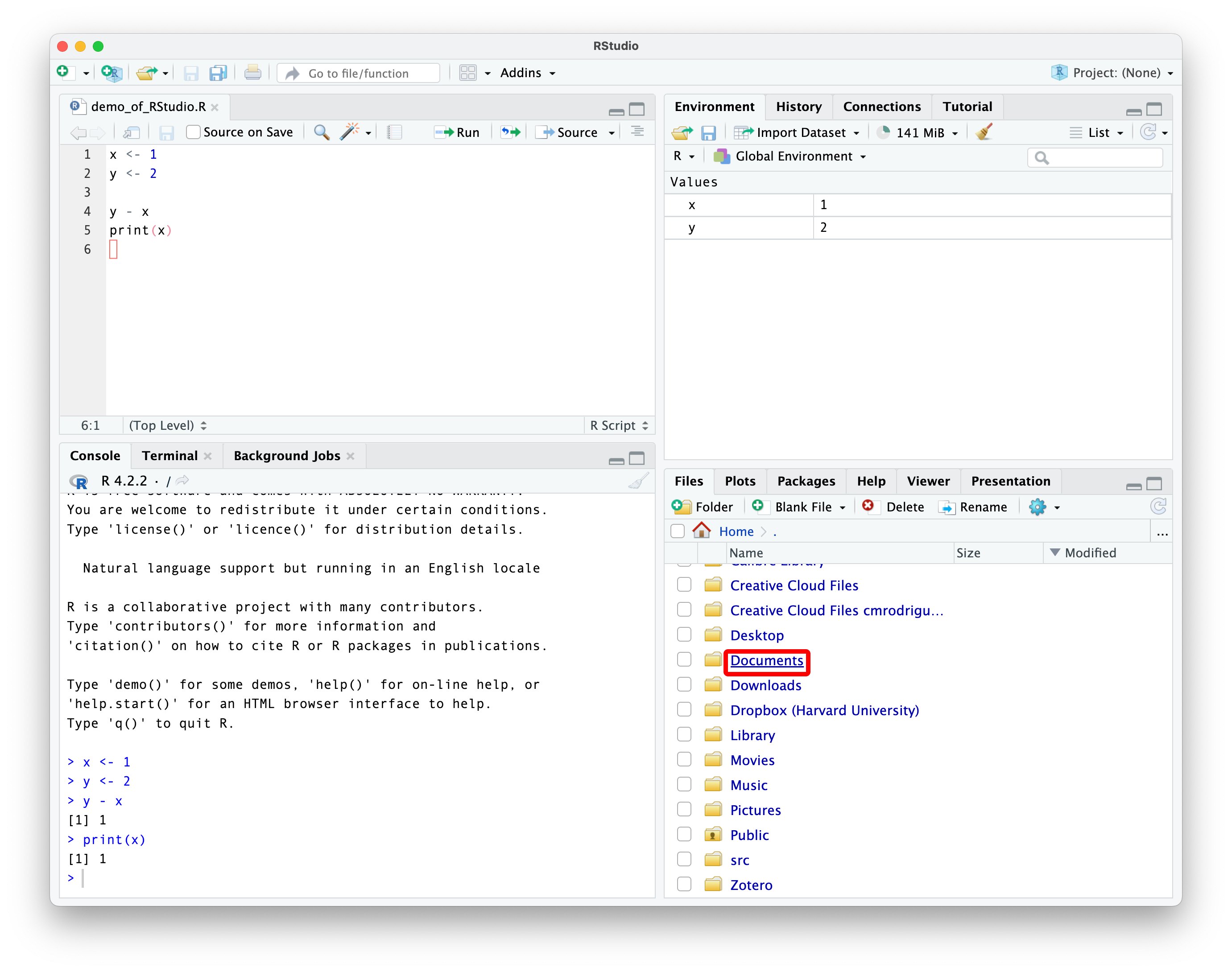
navigating using the file pane
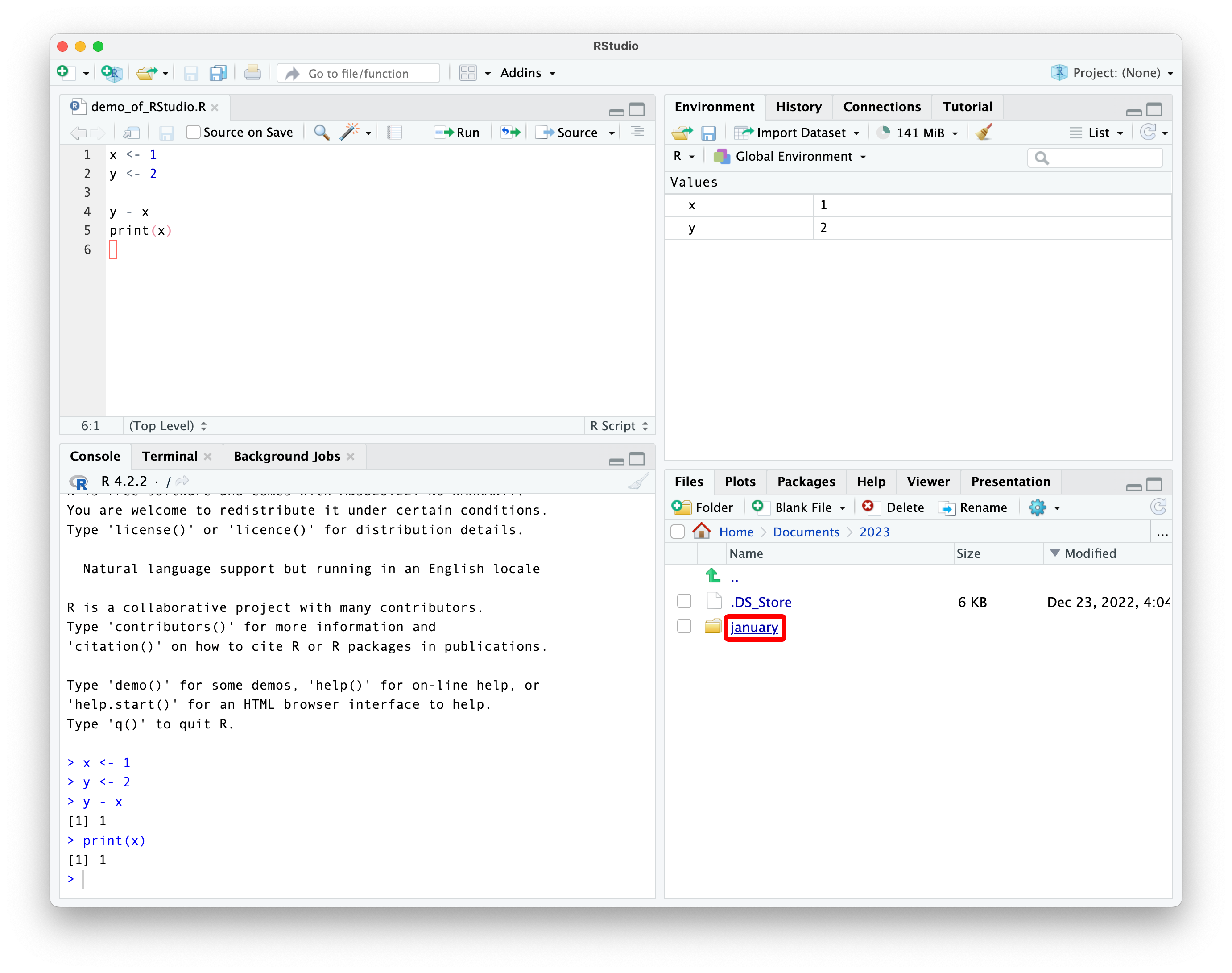
notice the path to the folder shown
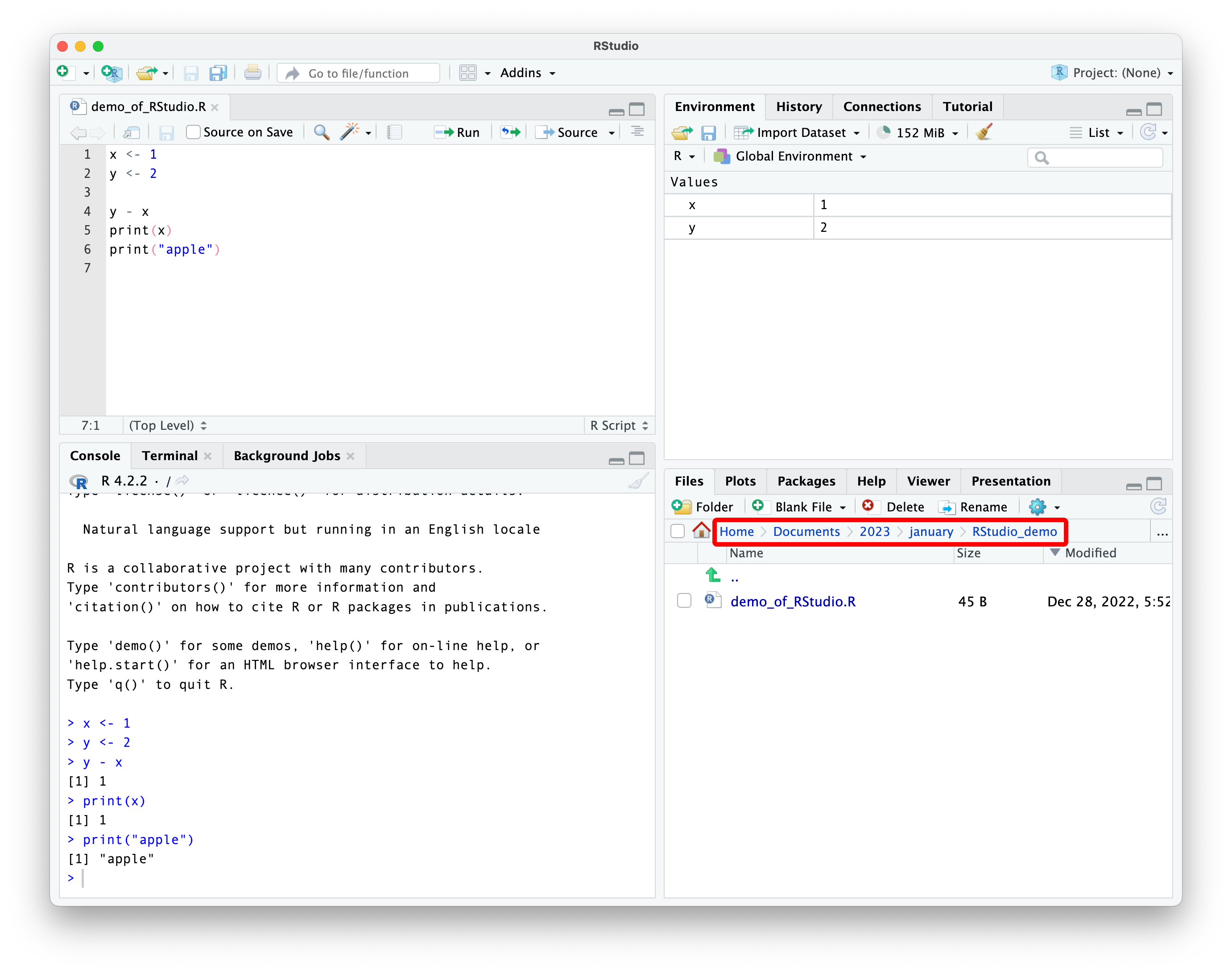
pay attention to your working directory
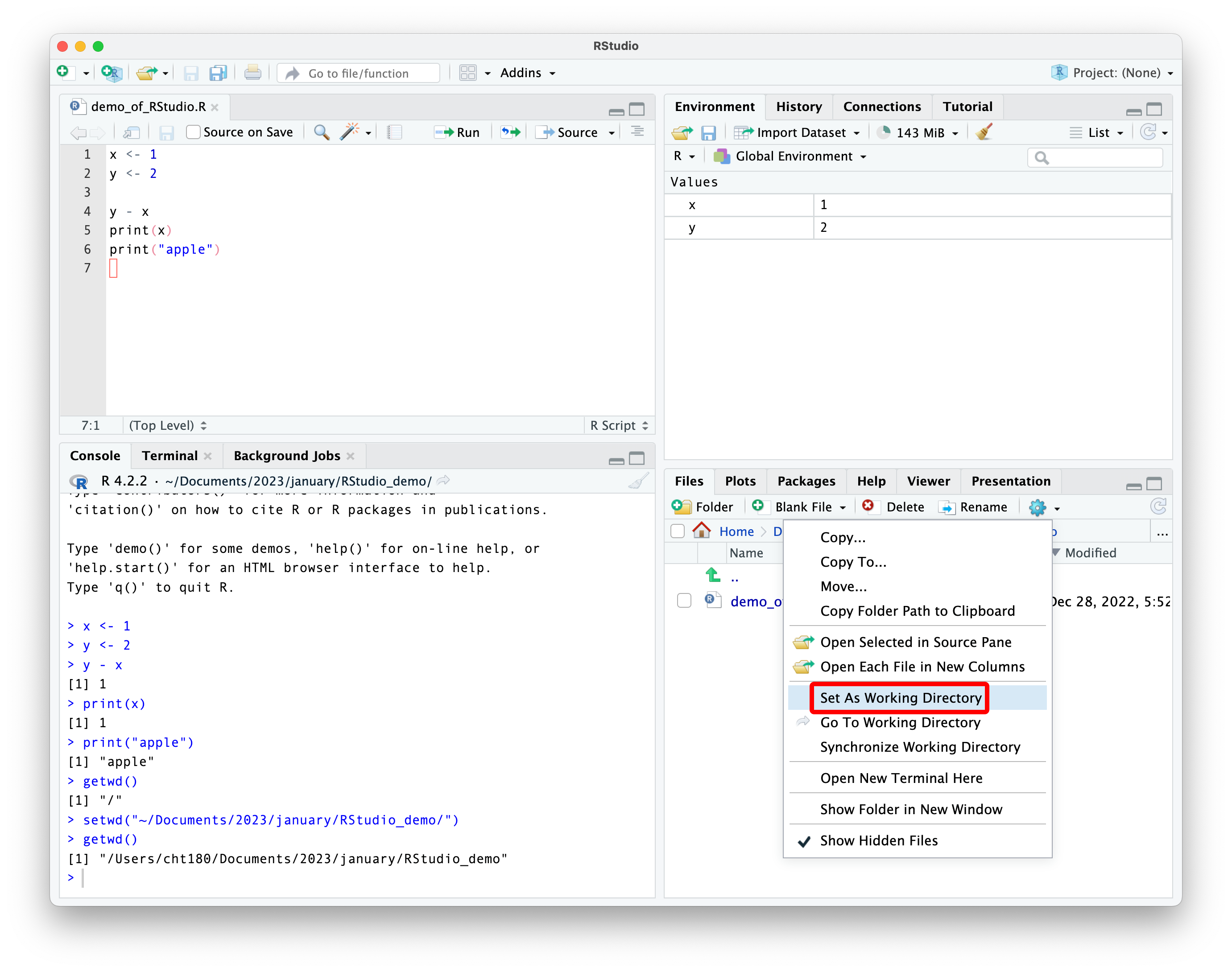
what is a working directory?
the working directory is the default location where R will look for files you want to load and where it will save files.
example: let’s say your working directory is C:/Users/me/Documents/ and you instruct R to load file.txt — then R will look for file.txt in C:/Users/me/Documents/. you can also use full paths, so you can tell R that instead it should load C:/Users/me/Documents/specific_folder/file.txt.
the difference between file.txt vs. C:/Users/me/Documents/specific_folder/file.txt is that the first is a relative path (relative to the working directory) and the second is an absolute path.
you can think of the working directory as “what folder does R have open right now?”
you can set the working directory through commands
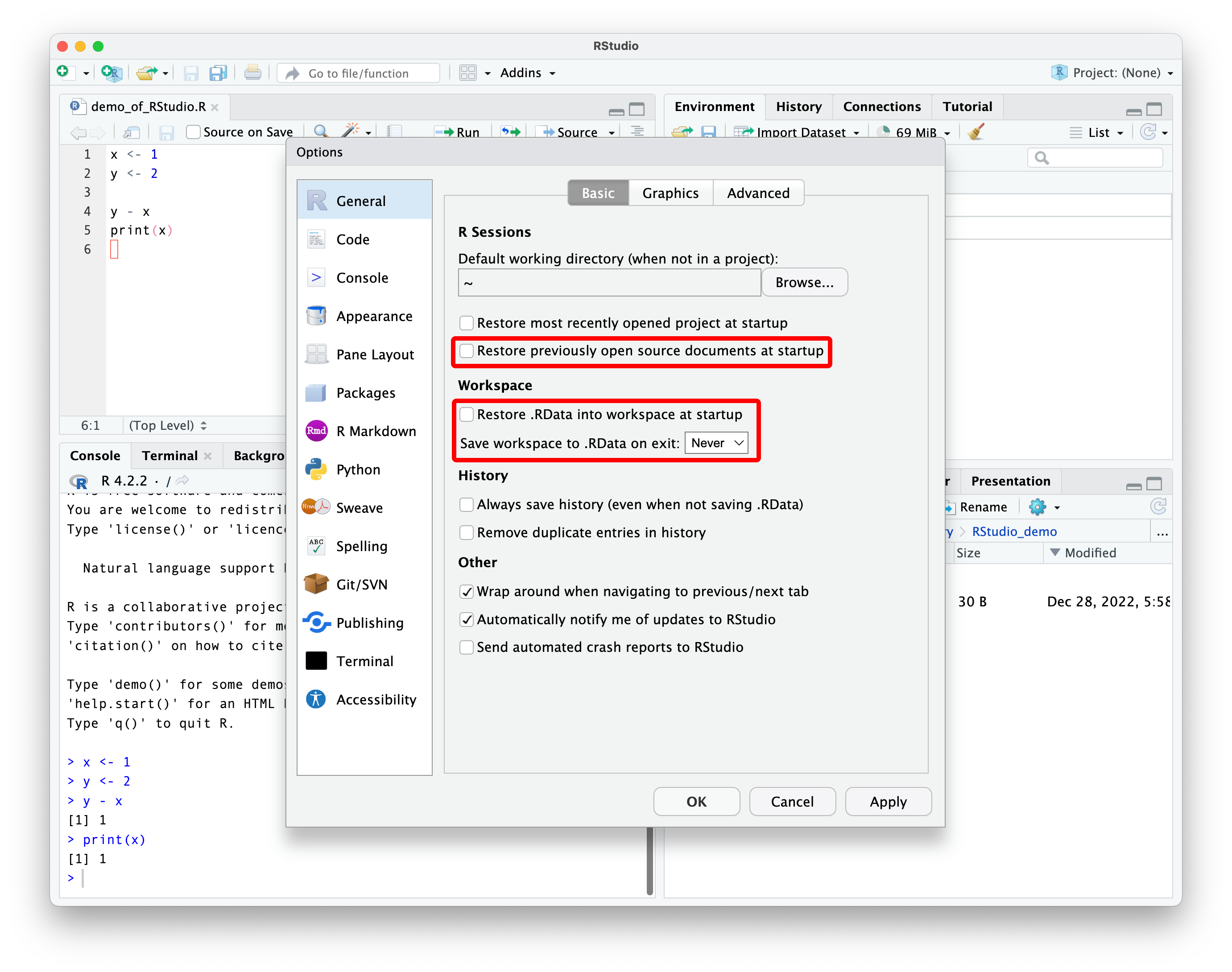
some helpful settings
highly suggested settings to disable
dark mode / other themes
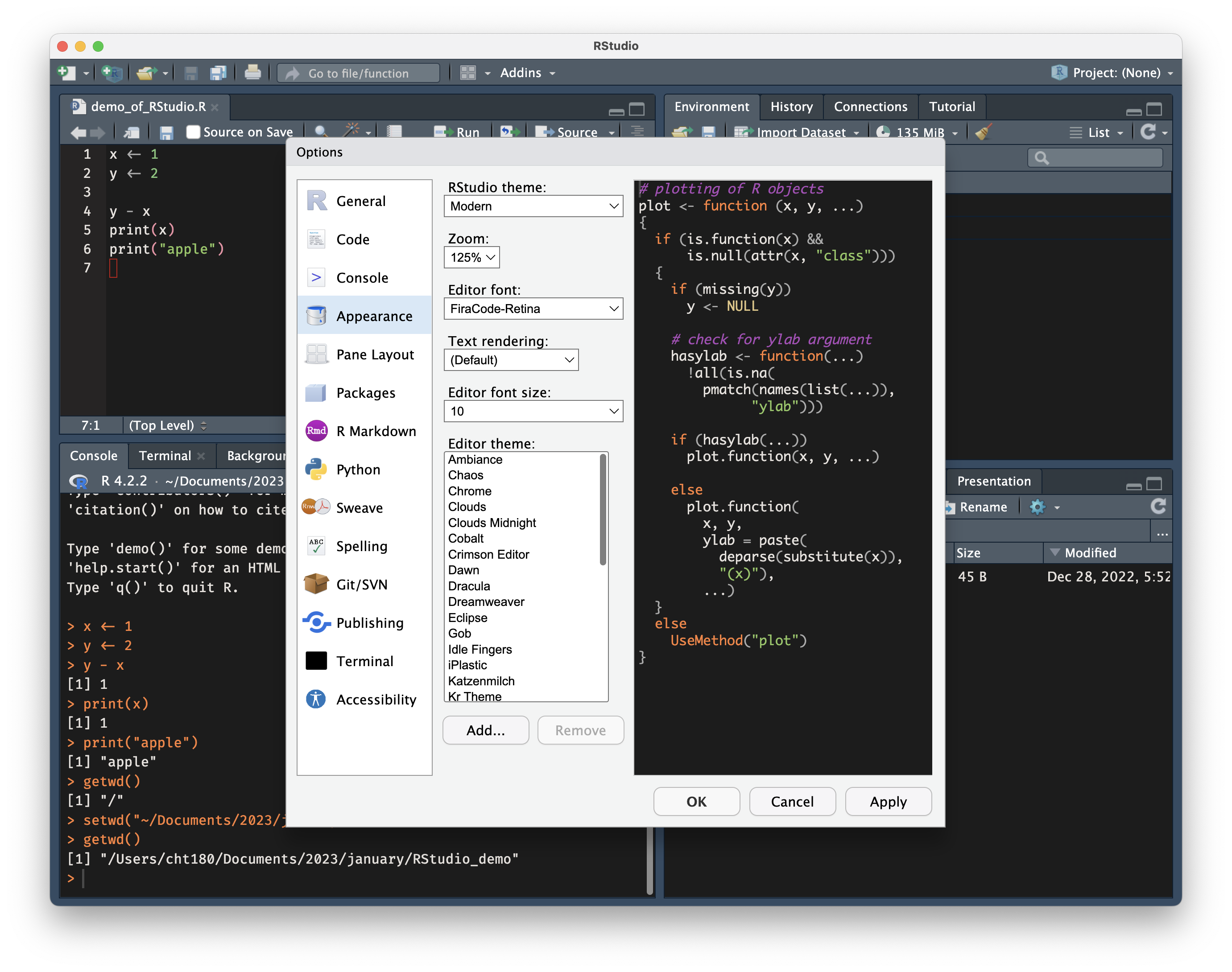
dark mode / other themes
keyboard shortcuts
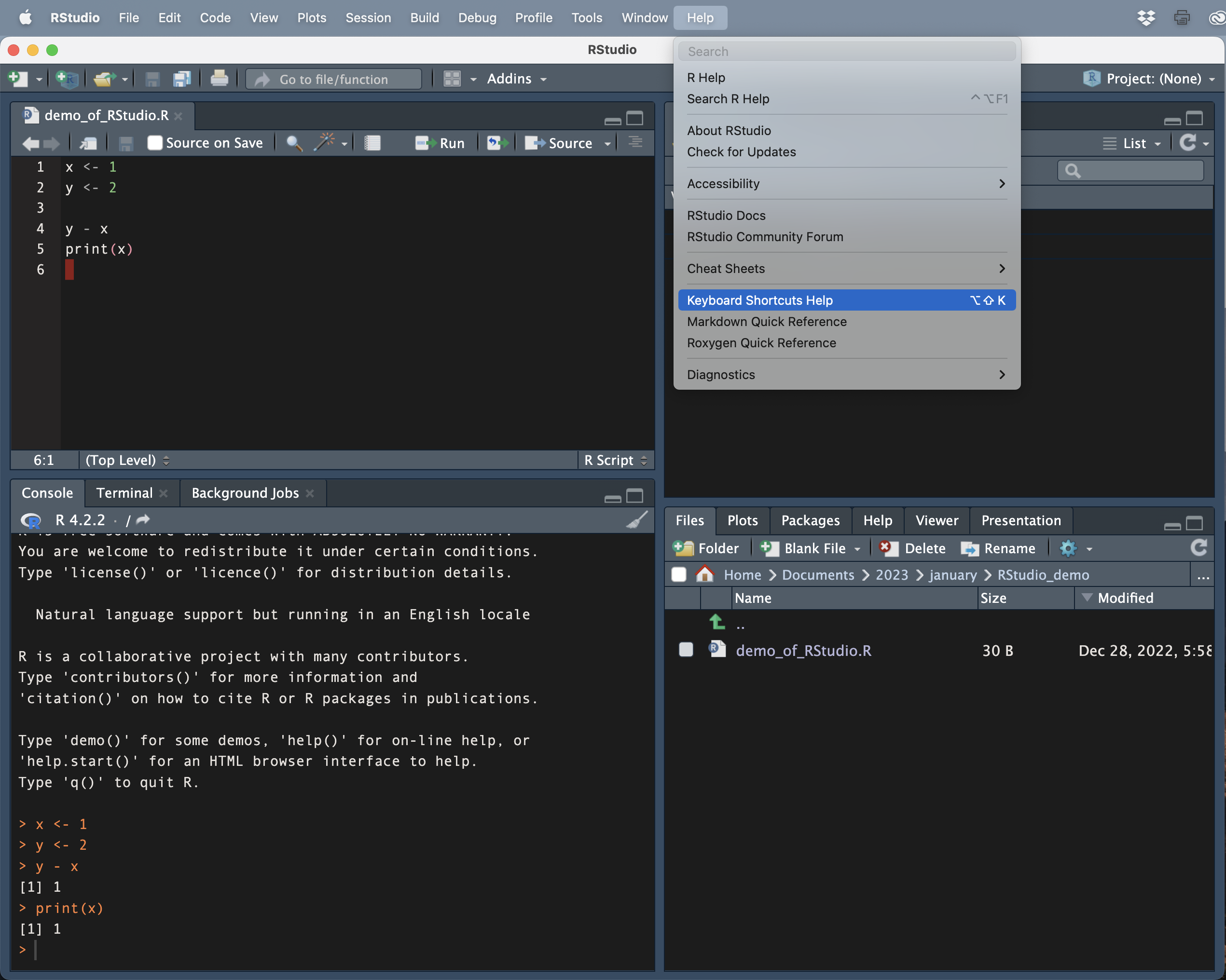
keyboard shortcuts
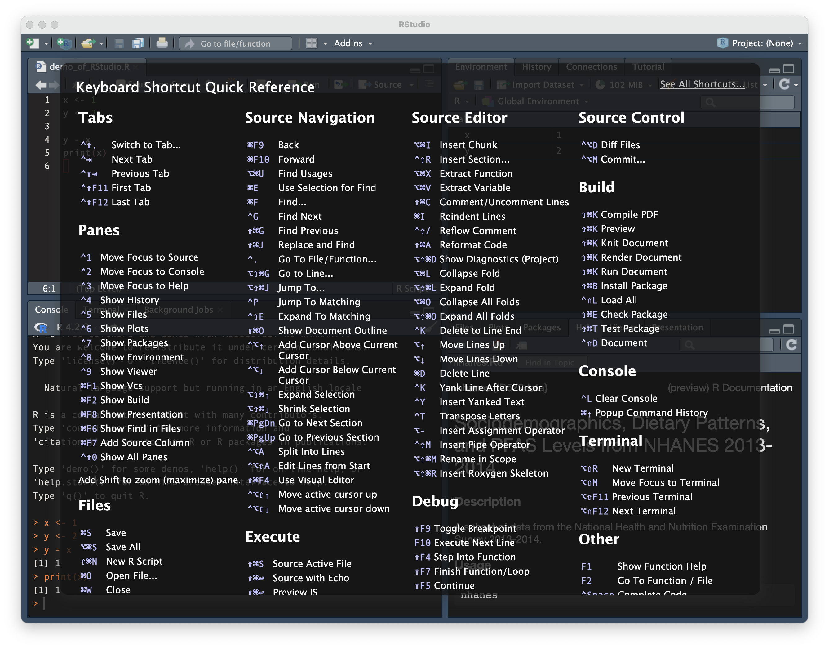
keyboard shortcuts
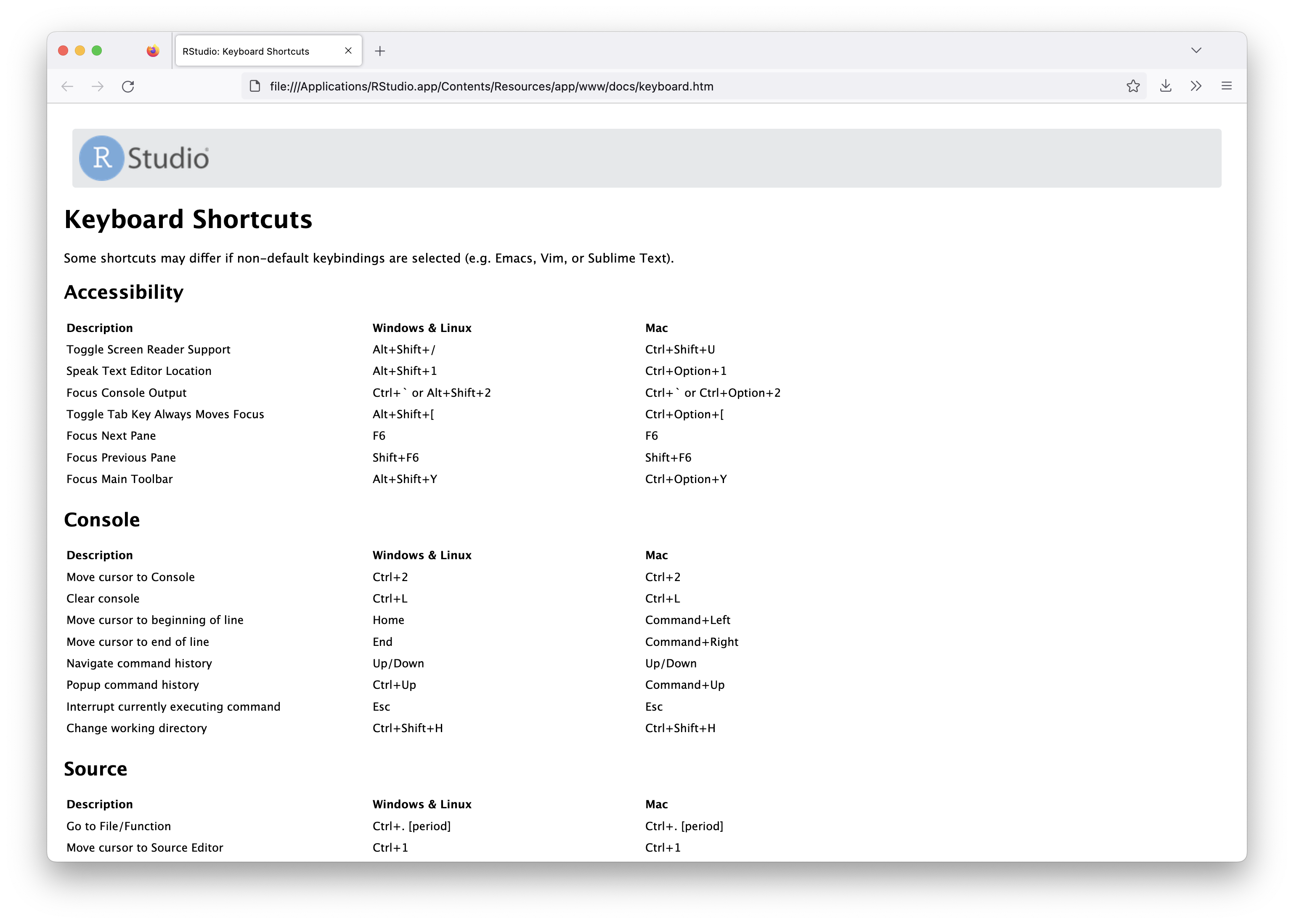
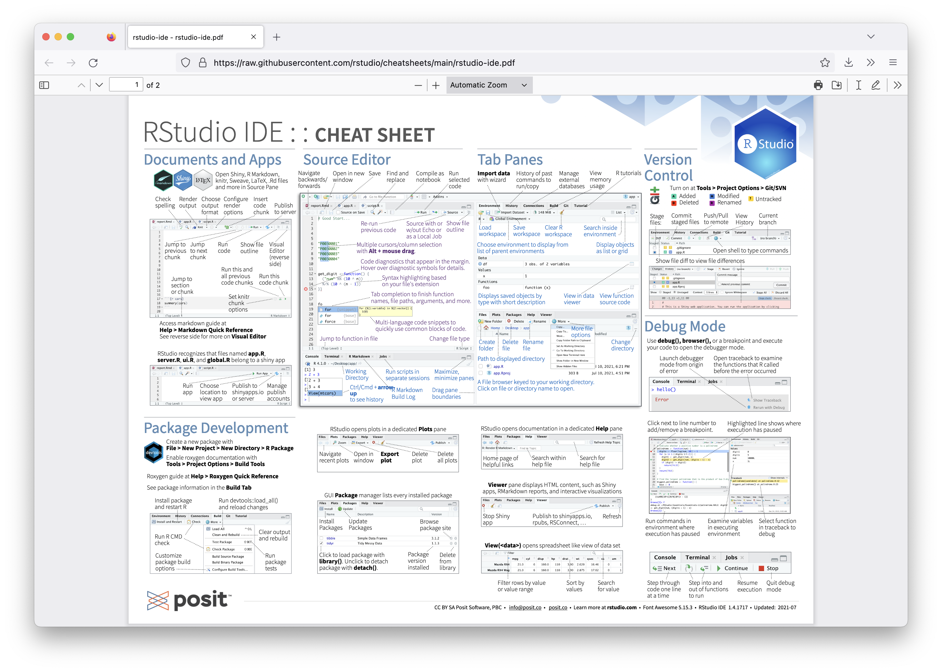
RStudio IDE cheatsheet
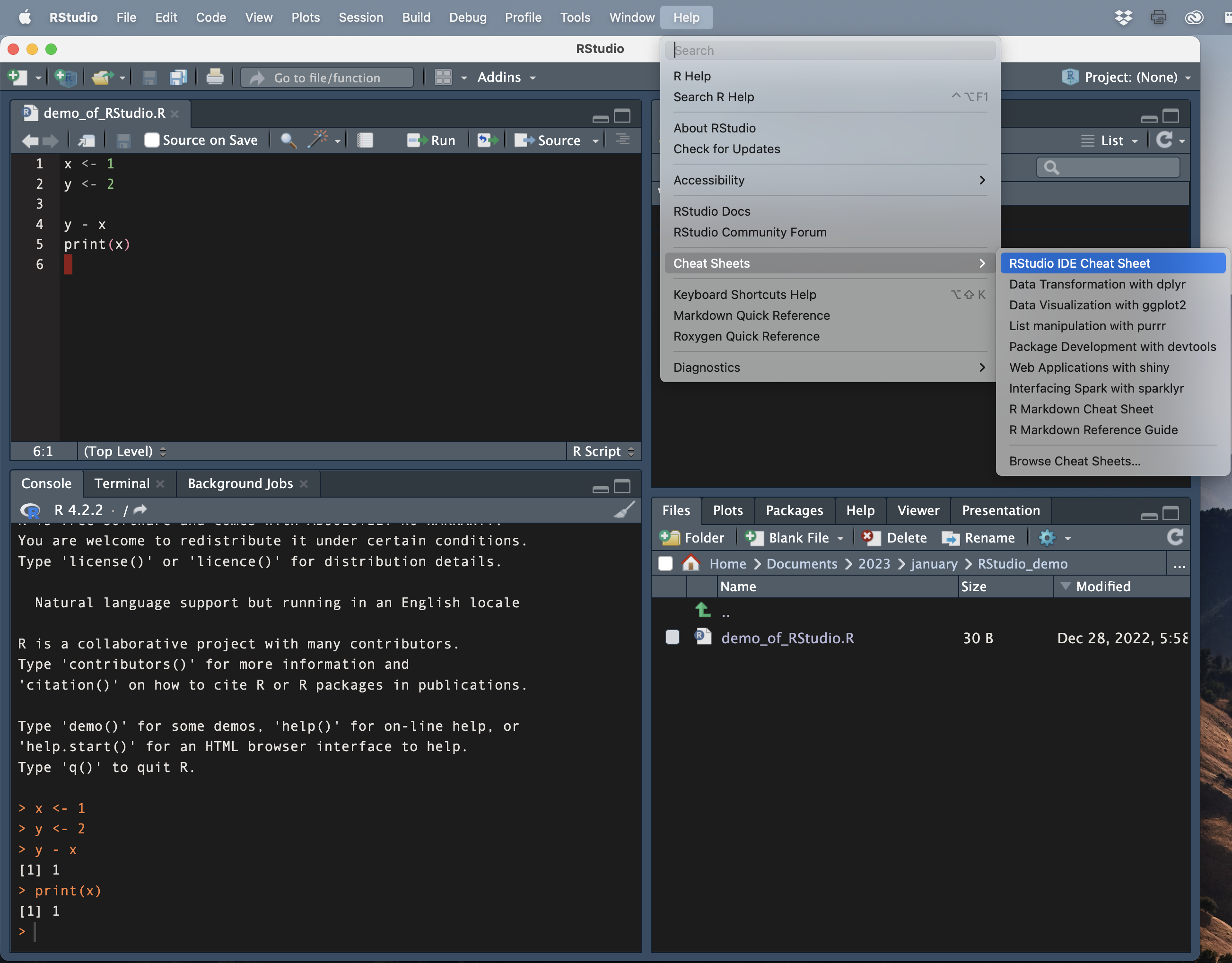
RStudio IDE cheatsheet
basics of R
arithmetic
The usual arithmetic operators you’re familiar with are available to you
arithmetic functions
assigning variables
vectors
vectors create combinations of multiple values which are all of the same type (i.e., one of numeric, character, or logical).
in fancy computer science language, we would say this makes vectors a homogeneous data structure.
- create a vector using
c()for concatenate - for missing data, use
NA(not available/not applicable) orNaN(not a number) - extract individual items using
my_vector[i]to get the ith element - calculate statistics on vectors with:
max(x),min(x),range(x),length(x),sum(x),mean(x),prod(x),sd(x),var(x),sort(x),summary(x)
an example working with vectors
factors
one particularly important type of vector is a factor, which is used to store categorical variables where values are repeated frequently and there is a pre-specified set of distinct levels.
# create a factor: let's say we have a study with 5 participants
study_participant_genders <- factor(
  c('non-binary',
    'transgender female',
    'non-binary',
    'cis female',
    'transgender female'))

# create a frequency table
table(study_participant_genders)
#> study_participant_genders
#>         cis female         non-binary transgender female
#>                  1                  2                  2

# get a list of the distinct levels
levels(study_participant_genders)
#> [1] "cis female"         "non-binary"         "transgender female"
lists
lists are an important heterogeneous data structure
create a list using list(), extract elements from it using my_list[[i]] to get the ith element from it, or use the my_list$element_name syntax if the elements in the list are named.
data frames
data frames are a data structure composed of multiple columns of data, all of which have the same length, but which may differ in type.
here’s an example:
data frames will be the most important data structure in this class!
as you might have guessed, the corresponding fancy computer science lingo would be to say that data frames are a heterogeneous data structure.
matrices
matrices are data structures made up of columns of data, all of the same type, all with the same length.
some functions to use with matrices
- to create matrices, use:
matrix(),cbind(),rbind() - to name their rows or columns:
rownames()andcolnames() - to check and convert:
is.matrix()andas.matrix() - transpose a matrix:
t() - get dimensions:
ncol()nrow(),dim() - subset a matrix:
my_matrix[row, col] - calculations with numeric matrices:
rowSums(),colSums(),rowMeans(),colMeans()
matrices

pup_stats <- matrix(
  data = c(
  3.8, 3.6, 3.7, 3.8, 3.5,     # 1st column
  8.5,   6, 7.7,   8, 8.2,     # 2nd column
  1,    .9, 1.2, 1.1,  .9),    # 3rd column
  ncol = 3, nrow = 5)

colnames(pup_stats) <-
  c('body_length_ft',
  'ear_width_in',
  'nose_width_in')

rownames(pup_stats) <-
  c('hodu',
    'coco-chanel',
    'sabre',
    'kissy',
'mochi')installing packages
R packages are extensions to the R programming language that contain code, data, and documentation.
R packages provide reusable R functions, documentation on how to use them, tests, and sample data.
# to install a package from CRAN use install.packages("packageName") with quotes
install.packages("tidyverse")
#> trying URL 'https://cloud.r-project.org/bin/macosx/big-sur-arm64/contrib/4.2/tidyverse_1.3.2.tgz'
#> Content type 'application/x-gzip' length 425892 bytes (415 KB)
#> ==================================================
#> downloaded 415 KB
#>
#>
#> The downloaded binary packages are in
#>  /var/folders/m8/2_hpqf1n5g3__1ps7nn8t31r0000gn/T//RtmpxHXjRQ/downloaded_packages
CRAN is the Comprehensive R Archive Network which acts to guarantee that packages downloaded from CRAN will compile, have documentation, and follow conventional norms about how packages should work.
installing packages
packages can also be installed from GitHub repositories using the {devtools} package.
loading packages
# to load a package use library(packageName) without quotes

library(tidyverse)
#> ── Attaching packages ───────────────────────────────────────────────────────────────────────────── tidyverse 1.3.2 ──
#> ✔ ggplot2 3.3.6     ✔ purrr   0.3.4
#> ✔ tibble  3.1.7     ✔ dplyr   1.0.9
#> ✔ tidyr   1.2.0     ✔ stringr 1.4.0
#> ✔ readr   2.1.2     ✔ forcats 0.5.1
#> ── Conflicts ──────────────────────────────────────────────────────────────────────────────── tidyverse_conflicts() ──
#> ✖ dplyr::filter() masks stats::filter()
#> ✖ dplyr::lag()    masks stats::lag()
getting help
Use help() or ? to get help on a specific function.
help(mean) # or run ?mean
#> mean                   package:base                    R Documentation
#>
#> Arithmetic Mean
#>
#> Description:
#>
#>      Generic function for the (trimmed) arithmetic mean.
#>
#> Usage:
#>
#>      mean(x, ...)
#>
#>      ## Default S3 method:
#>      mean(x, trim = 0, na.rm = FALSE, ...)
#> Arguments:
#>
#>        x: An R object.  Currently there are methods for numeric/logical
#>           vectors and date, date-time and time interval objects.
#>           Complex vectors are allowed for ‘trim = 0’, only.
#>
#>     trim: the fraction (0 to 0.5) of observations to be trimmed from
#>           each end of ‘x’ before the mean is computed.  Values of trim
#>           outside that range are taken as the nearest endpoint.
#>
#>    na.rm: a logical evaluating to ‘TRUE’ or ‘FALSE’ indicating whether
#>           ‘NA’ values should be stripped before the computation
#>           proceeds.
#>
#>      ...: further arguments passed to or from other methods.
#>
#> Value:
#>
#>      If ‘trim’ is zero (the default), the arithmetic mean of the values
#>      in ‘x’ is computed, as a numeric or complex vector of length one.
#>      If ‘x’ is not logical (coerced to numeric), numeric (including
#>      integer) or complex, ‘NA_real_’ is returned, with a warning.
#>
#>      If ‘trim’ is non-zero, a symmetrically trimmed mean is computed
#>      with a fraction of ‘trim’ observations deleted from each end
#>      before the mean is computed.
#>
#> References:
#>
#>      Becker, R. A., Chambers, J. M. and Wilks, A. R. (1988) _The New S
#>      Language_.  Wadsworth & Brooks/Cole.
#>
#> See Also:
#>
#>      ‘weighted.mean’, ‘mean.POSIXct’, ‘colMeans’ for row and column
#>      means.
#> Examples:
#>
#>      x <- c(0:10, 50)
#>      xm <- mean(x)
#>      c(xm, mean(x, trim = 0.10))
getting help
Using the help() command for most functions is straightforward, but there are situations where you need to be a little bit careful.
- if you are looking for help for a function from a specific package, especially where that function appears in multiple packages, you should run
help(filter, package='dplyr'). - if you’re trying to get help on a function in R that is a symbol, like the arithmetic operators (
/,+,-,*,^), or the assignment operator<-, then you should put it in quotes when you call help:help("*") - there’s more advice on getting help from inside R here:
https://www.r-project.org/help.html
builtin example datasets
there are a handful of builtin example datasets you can use to test out ideas on.
                     mpg cyl  disp  hp drat    wt  qsec vs am gear carb
Mazda RX4           21.0   6 160.0 110 3.90 2.620 16.46  0  1    4    4
Mazda RX4 Wag       21.0   6 160.0 110 3.90 2.875 17.02  0  1    4    4
Datsun 710          22.8   4 108.0  93 3.85 2.320 18.61  1  1    4    1
Hornet 4 Drive      21.4   6 258.0 110 3.08 3.215 19.44  1  0    3    1
Hornet Sportabout   18.7   8 360.0 175 3.15 3.440 17.02  0  0    3    2
Valiant             18.1   6 225.0 105 2.76 3.460 20.22  1  0    3    1
Duster 360          14.3   8 360.0 245 3.21 3.570 15.84  0  0    3    4
Merc 240D           24.4   4 146.7  62 3.69 3.190 20.00  1  0    4    2
Merc 230            22.8   4 140.8  95 3.92 3.150 22.90  1  0    4    2
Merc 280            19.2   6 167.6 123 3.92 3.440 18.30  1  0    4    4
Merc 280C           17.8   6 167.6 123 3.92 3.440 18.90  1  0    4    4
Merc 450SE          16.4   8 275.8 180 3.07 4.070 17.40  0  0    3    3
Merc 450SL          17.3   8 275.8 180 3.07 3.730 17.60  0  0    3    3
Merc 450SLC         15.2   8 275.8 180 3.07 3.780 18.00  0  0    3    3
Cadillac Fleetwood  10.4   8 472.0 205 2.93 5.250 17.98  0  0    3    4
Lincoln Continental 10.4   8 460.0 215 3.00 5.424 17.82  0  0    3    4
Chrysler Imperial   14.7   8 440.0 230 3.23 5.345 17.42  0  0    3    4
Fiat 128            32.4   4  78.7  66 4.08 2.200 19.47  1  1    4    1
Honda Civic         30.4   4  75.7  52 4.93 1.615 18.52  1  1    4    2
Toyota Corolla      33.9   4  71.1  65 4.22 1.835 19.90  1  1    4    1
Toyota Corona       21.5   4 120.1  97 3.70 2.465 20.01  1  0    3    1
Dodge Challenger    15.5   8 318.0 150 2.76 3.520 16.87  0  0    3    2
AMC Javelin         15.2   8 304.0 150 3.15 3.435 17.30  0  0    3    2
Camaro Z28          13.3   8 350.0 245 3.73 3.840 15.41  0  0    3    4
Pontiac Firebird    19.2   8 400.0 175 3.08 3.845 17.05  0  0    3    2
Fiat X1-9           27.3   4  79.0  66 4.08 1.935 18.90  1  1    4    1
Porsche 914-2       26.0   4 120.3  91 4.43 2.140 16.70  0  1    5    2
Lotus Europa        30.4   4  95.1 113 3.77 1.513 16.90  1  1    5    2
Ford Pantera L      15.8   8 351.0 264 4.22 3.170 14.50  0  1    5    4
Ferrari Dino        19.7   6 145.0 175 3.62 2.770 15.50  0  1    5    6
Maserati Bora       15.0   8 301.0 335 3.54 3.570 14.60  0  1    5    8
Volvo 142E          21.4   4 121.0 109 4.11 2.780 18.60  1  1    4    2
Sepal.Length Sepal.Width Petal.Length Petal.Width Species
5.1 3.5 1.4 0.2 setosa
4.9 3.0 1.4 0.2 setosa
4.7 3.2 1.3 0.2 setosa
4.6 3.1 1.5 0.2 setosa
5.0 3.6 1.4 0.2 setosa
5.4 3.9 1.7 0.4 setosa
4.6 3.4 1.4 0.3 setosa
5.0 3.4 1.5 0.2 setosa
4.4 2.9 1.4 0.2 setosa
4.9 3.1 1.5 0.1 setosa
5.4 3.7 1.5 0.2 setosa
4.8 3.4 1.6 0.2 setosa
4.8 3.0 1.4 0.1 setosa
4.3 3.0 1.1 0.1 setosa
5.8 4.0 1.2 0.2 setosa
5.7 4.4 1.5 0.4 setosa
5.4 3.9 1.3 0.4 setosa
5.1 3.5 1.4 0.3 setosa
5.7 3.8 1.7 0.3 setosa
5.1 3.8 1.5 0.3 setosa
5.4 3.4 1.7 0.2 setosa
5.1 3.7 1.5 0.4 setosa
4.6 3.6 1.0 0.2 setosa
5.1 3.3 1.7 0.5 setosa
4.8 3.4 1.9 0.2 setosa
5.0 3.0 1.6 0.2 setosa
5.0 3.4 1.6 0.4 setosa
5.2 3.5 1.5 0.2 setosa
5.2 3.4 1.4 0.2 setosa
4.7 3.2 1.6 0.2 setosa
4.8 3.1 1.6 0.2 setosa
5.4 3.4 1.5 0.4 setosa
5.2 4.1 1.5 0.1 setosa
5.5 4.2 1.4 0.2 setosa
4.9 3.1 1.5 0.2 setosa
5.0 3.2 1.2 0.2 setosa
5.5 3.5 1.3 0.2 setosa
4.9 3.6 1.4 0.1 setosa
4.4 3.0 1.3 0.2 setosa
5.1 3.4 1.5 0.2 setosa
5.0 3.5 1.3 0.3 setosa
4.5 2.3 1.3 0.3 setosa
4.4 3.2 1.3 0.2 setosa
5.0 3.5 1.6 0.6 setosa
5.1 3.8 1.9 0.4 setosa
4.8 3.0 1.4 0.3 setosa
5.1 3.8 1.6 0.2 setosa
4.6 3.2 1.4 0.2 setosa
5.3 3.7 1.5 0.2 setosa
5.0 3.3 1.4 0.2 setosa
7.0 3.2 4.7 1.4 versicolor
6.4 3.2 4.5 1.5 versicolor
6.9 3.1 4.9 1.5 versicolor
5.5 2.3 4.0 1.3 versicolor
6.5 2.8 4.6 1.5 versicolor
5.7 2.8 4.5 1.3 versicolor
6.3 3.3 4.7 1.6 versicolor
4.9 2.4 3.3 1.0 versicolor
6.6 2.9 4.6 1.3 versicolor
5.2 2.7 3.9 1.4 versicolor
5.0 2.0 3.5 1.0 versicolor
5.9 3.0 4.2 1.5 versicolor
6.0 2.2 4.0 1.0 versicolor
6.1 2.9 4.7 1.4 versicolor
5.6 2.9 3.6 1.3 versicolor
6.7 3.1 4.4 1.4 versicolor
5.6 3.0 4.5 1.5 versicolor
5.8 2.7 4.1 1.0 versicolor
6.2 2.2 4.5 1.5 versicolor
5.6 2.5 3.9 1.1 versicolor
5.9 3.2 4.8 1.8 versicolor
6.1 2.8 4.0 1.3 versicolor
6.3 2.5 4.9 1.5 versicolor
6.1 2.8 4.7 1.2 versicolor
6.4 2.9 4.3 1.3 versicolor
6.6 3.0 4.4 1.4 versicolor
6.8 2.8 4.8 1.4 versicolor
6.7 3.0 5.0 1.7 versicolor
6.0 2.9 4.5 1.5 versicolor
5.7 2.6 3.5 1.0 versicolor
5.5 2.4 3.8 1.1 versicolor
5.5 2.4 3.7 1.0 versicolor
5.8 2.7 3.9 1.2 versicolor
6.0 2.7 5.1 1.6 versicolor
5.4 3.0 4.5 1.5 versicolor
6.0 3.4 4.5 1.6 versicolor
6.7 3.1 4.7 1.5 versicolor
6.3 2.3 4.4 1.3 versicolor
5.6 3.0 4.1 1.3 versicolor
5.5 2.5 4.0 1.3 versicolor
5.5 2.6 4.4 1.2 versicolor
6.1 3.0 4.6 1.4 versicolor
5.8 2.6 4.0 1.2 versicolor
5.0 2.3 3.3 1.0 versicolor
5.6 2.7 4.2 1.3 versicolor
5.7 3.0 4.2 1.2 versicolor
5.7 2.9 4.2 1.3 versicolor
6.2 2.9 4.3 1.3 versicolor
5.1 2.5 3.0 1.1 versicolor
5.7 2.8 4.1 1.3 versicolor
6.3 3.3 6.0 2.5 virginica
5.8 2.7 5.1 1.9 virginica
7.1 3.0 5.9 2.1 virginica
6.3 2.9 5.6 1.8 virginica
6.5 3.0 5.8 2.2 virginica
7.6 3.0 6.6 2.1 virginica
4.9 2.5 4.5 1.7 virginica
7.3 2.9 6.3 1.8 virginica
6.7 2.5 5.8 1.8 virginica
7.2 3.6 6.1 2.5 virginica
6.5 3.2 5.1 2.0 virginica
6.4 2.7 5.3 1.9 virginica
6.8 3.0 5.5 2.1 virginica
5.7 2.5 5.0 2.0 virginica
5.8 2.8 5.1 2.4 virginica
6.4 3.2 5.3 2.3 virginica
6.5 3.0 5.5 1.8 virginica
7.7 3.8 6.7 2.2 virginica
7.7 2.6 6.9 2.3 virginica
6.0 2.2 5.0 1.5 virginica
6.9 3.2 5.7 2.3 virginica
5.6 2.8 4.9 2.0 virginica
7.7 2.8 6.7 2.0 virginica
6.3 2.7 4.9 1.8 virginica
6.7 3.3 5.7 2.1 virginica
7.2 3.2 6.0 1.8 virginica
6.2 2.8 4.8 1.8 virginica
6.1 3.0 4.9 1.8 virginica
6.4 2.8 5.6 2.1 virginica
7.2 3.0 5.8 1.6 virginica
7.4 2.8 6.1 1.9 virginica
7.9 3.8 6.4 2.0 virginica
6.4 2.8 5.6 2.2 virginica
6.3 2.8 5.1 1.5 virginica
6.1 2.6 5.6 1.4 virginica
7.7 3.0 6.1 2.3 virginica
6.3 3.4 5.6 2.4 virginica
6.4 3.1 5.5 1.8 virginica
6.0 3.0 4.8 1.8 virginica
6.9 3.1 5.4 2.1 virginica
6.7 3.1 5.6 2.4 virginica
6.9 3.1 5.1 2.3 virginica
5.8 2.7 5.1 1.9 virginica
6.8 3.2 5.9 2.3 virginica
6.7 3.3 5.7 2.5 virginica
6.7 3.0 5.2 2.3 virginica
6.3 2.5 5.0 1.9 virginica
6.5 3.0 5.2 2.0 virginica
6.2 3.4 5.4 2.3 virginica
5.9 3.0 5.1 1.8 virginicadata packages
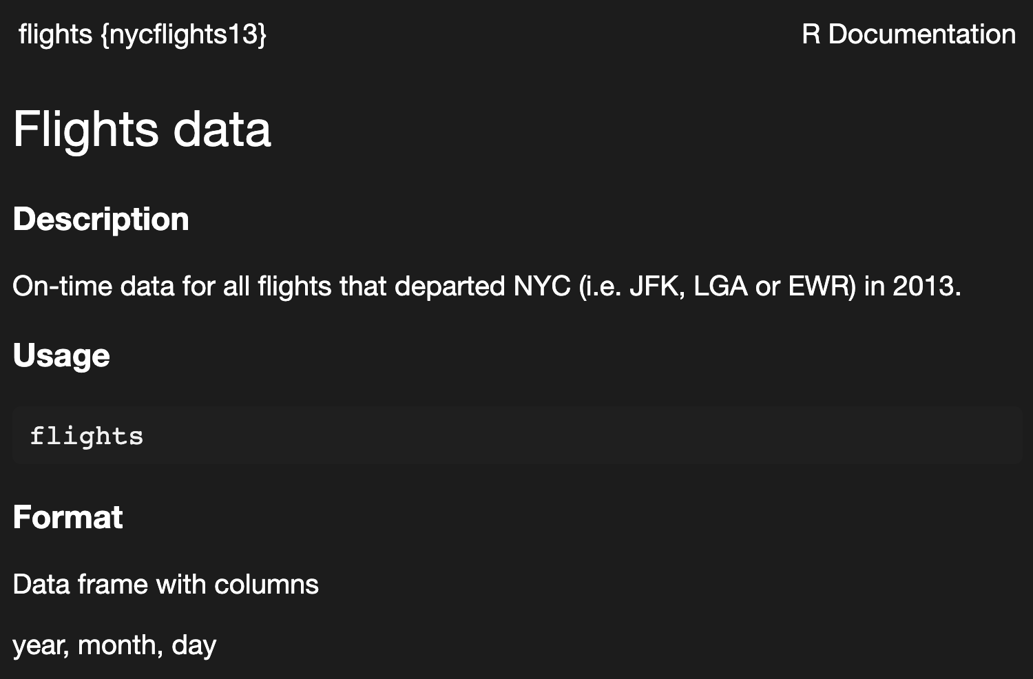
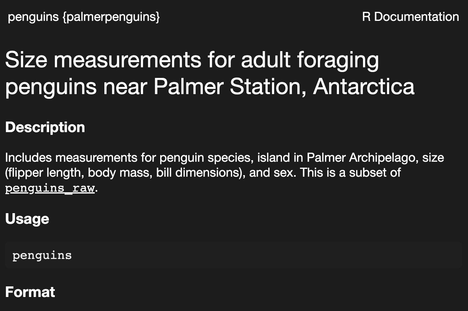
there are also packages that contain data; some that are particularly often referenced the {nycflights13} and {palmerpenguins} packages.
getting help
in this class, we are encouraging you to reference online materials including:
- R for Data Science Online Community https://www.rfordatasci.com/
- StackOverflow: https://stackoverflow.com/questions/tagged/r?tab=Votes
- the RStudio Community: https://community.rstudio.com/
- the /r/rstats reddit: https://www.reddit.com/r/rstats/
- twitter / mastodon: the #rstats hashtag, https://www.t4rstats.com/
- R Bloggers https://www.r-bloggers.com/
- Cross Validated: https://stats.stackexchange.com/questions?tab=Votes
learning how to help yourself learn R is one of the key skills we want you to take away from this class
key takeaways
- R and RStudio are available for you to download, for free
- the basic classes of data you should become familiar with are:
- numeric, character, logical
- the basic data structures you should become familiar with are:
- vectors, lists, data frames, matrices
- get help in R using
help()or?, or search online