
[1] "species"           "island"            "bill_length_mm"
[4] "bill_depth_mm"     "flipper_length_mm" "body_mass_g"
[7] "sex" "year" Amanda Hernandez (she/her)
hi there! I recently completed an MS in Environmental Health. I’m currently working in the public sector as a Presidential Management Fellow.
My master’s work was at the intersection of environmental geochemistry + public health, focused on addressing environmental health disparities through community-based participatory research and evidence-based decision-making.
I’m a self-taught R user, Shiny enthusiast, and advocate for coding in light mode.
Factor rules
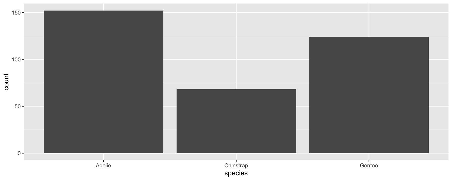
R by default returns your data in the order it occurs
Factors create an order and retain that order for all future uses of the variable
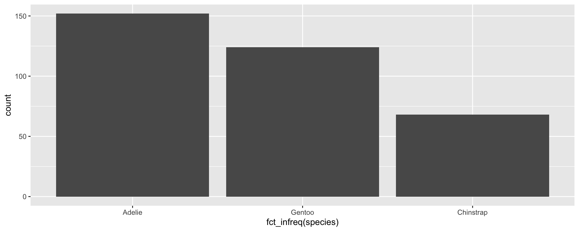
Changing the factor order: fct_infreq()
We may want to change the default factor order (alphabetical) and rearrange the order on the x axis. forcats:: gives us lots of options for rearranging our factors without having to manually list out all of the levels.
fct_infreq() allows us to sort by occurrence:
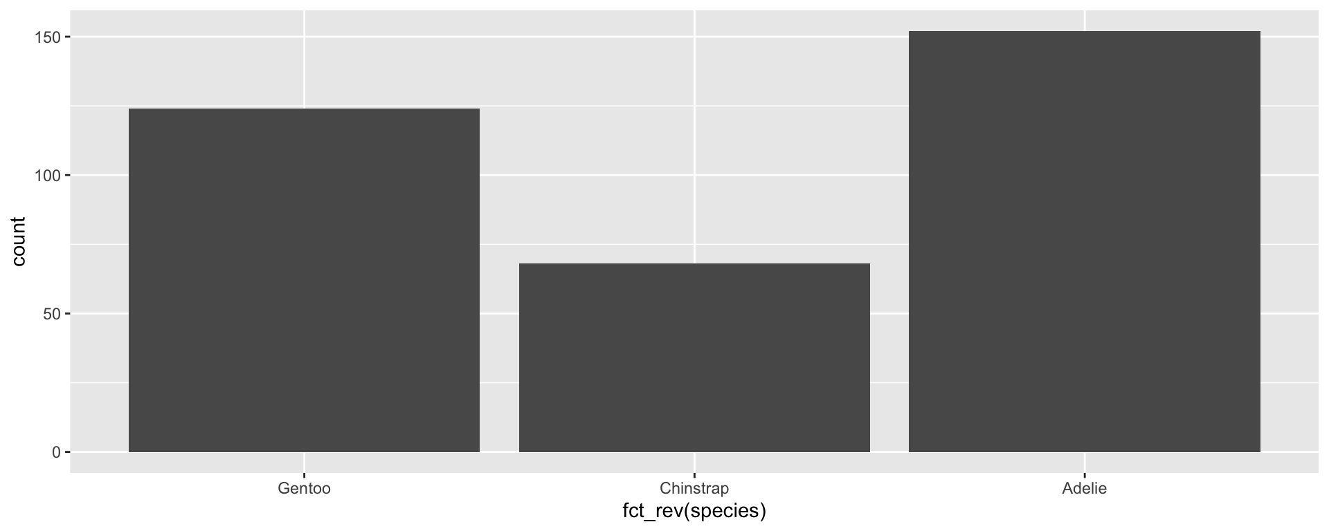
Changing the factor order: fct_rev()
fct_rev() flips the order in reverse

If you’re doing a lot of different analyses and visualization, you may want to change the factor order quite often.
Consider using these functions locally within your code so that you’re not actually changing the underlying dataset and future analyses.
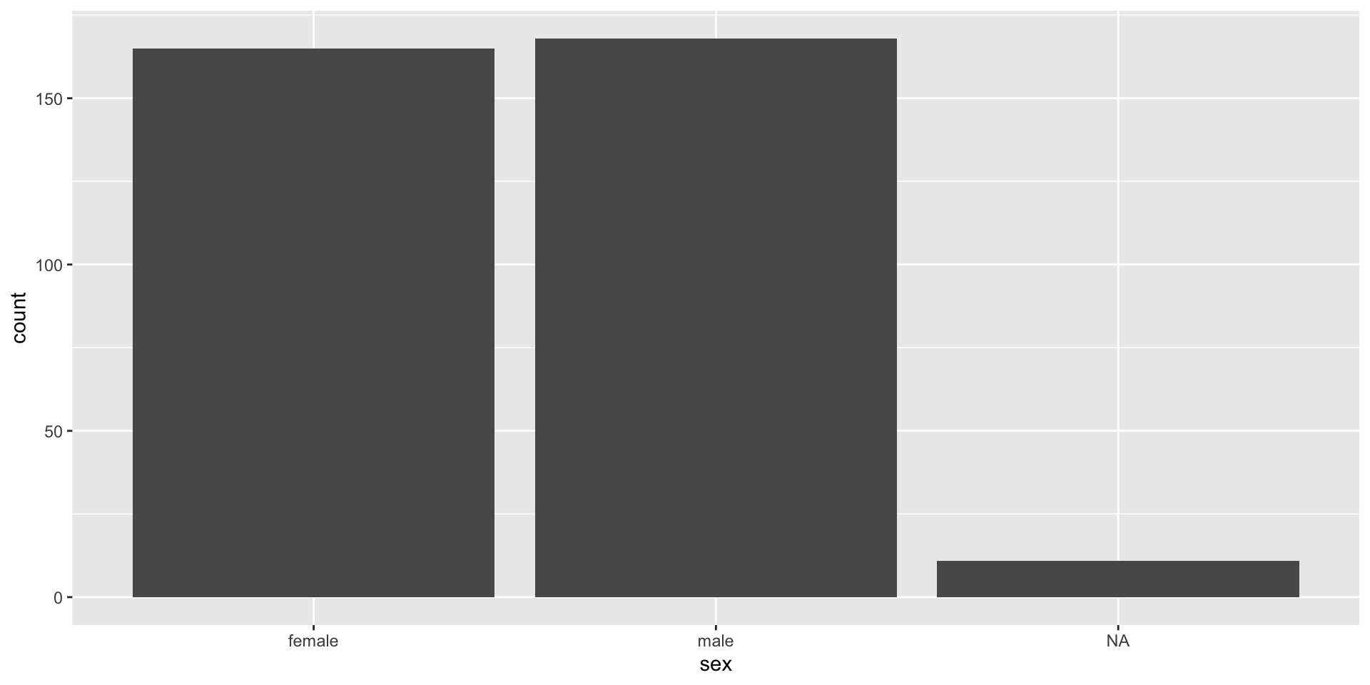
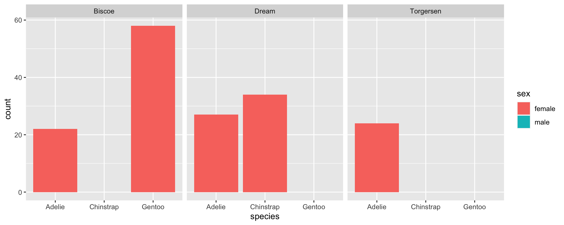
Factor rules: Missingness
Factor rules: Missingness
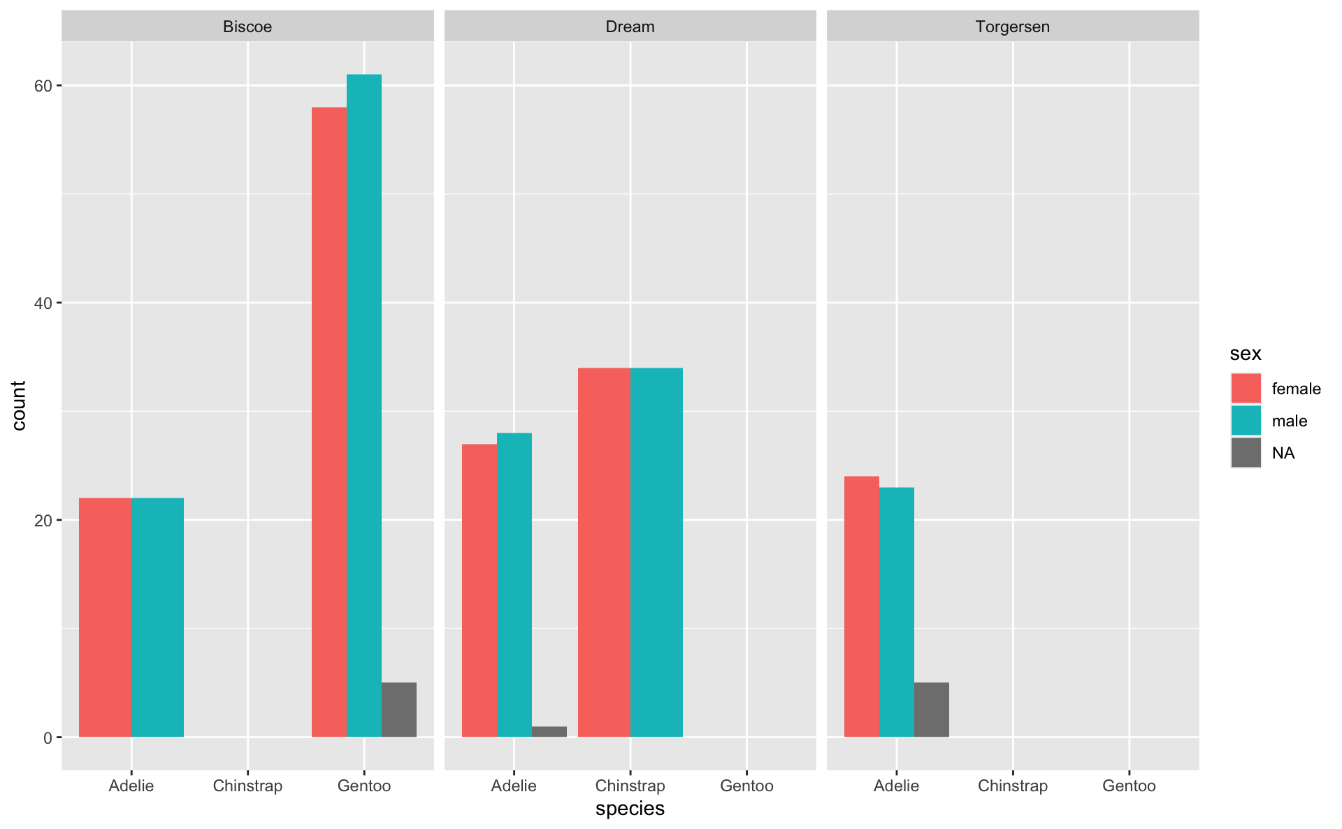
Empty groups + NAs in factors
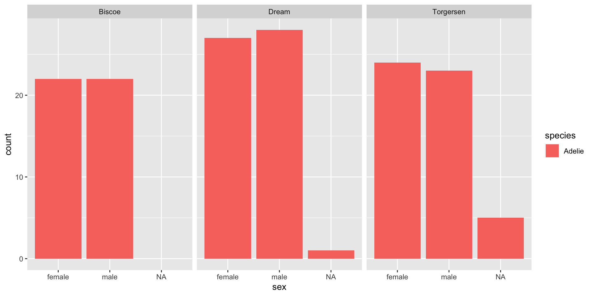
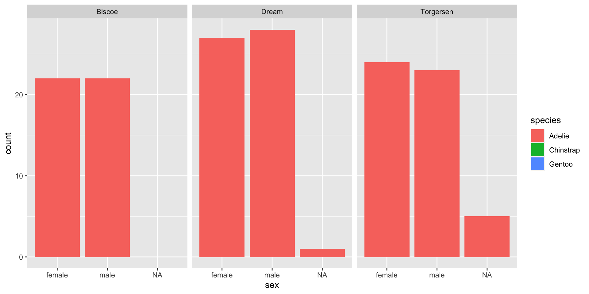
Empty groups + NAs in factors
- Remember: NAs are not considered a factor level, so if we filter out the NAs, they will not be included in the legend even if we specify to keep all levels.
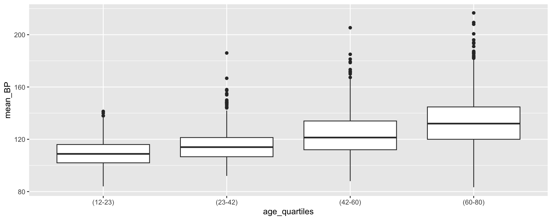
Creating age quartiles
   Min. 1st Qu.  Median    Mean 3rd Qu.    Max.
12.00 23.00 42.00 42.78 60.00 80.00 [1] "integer"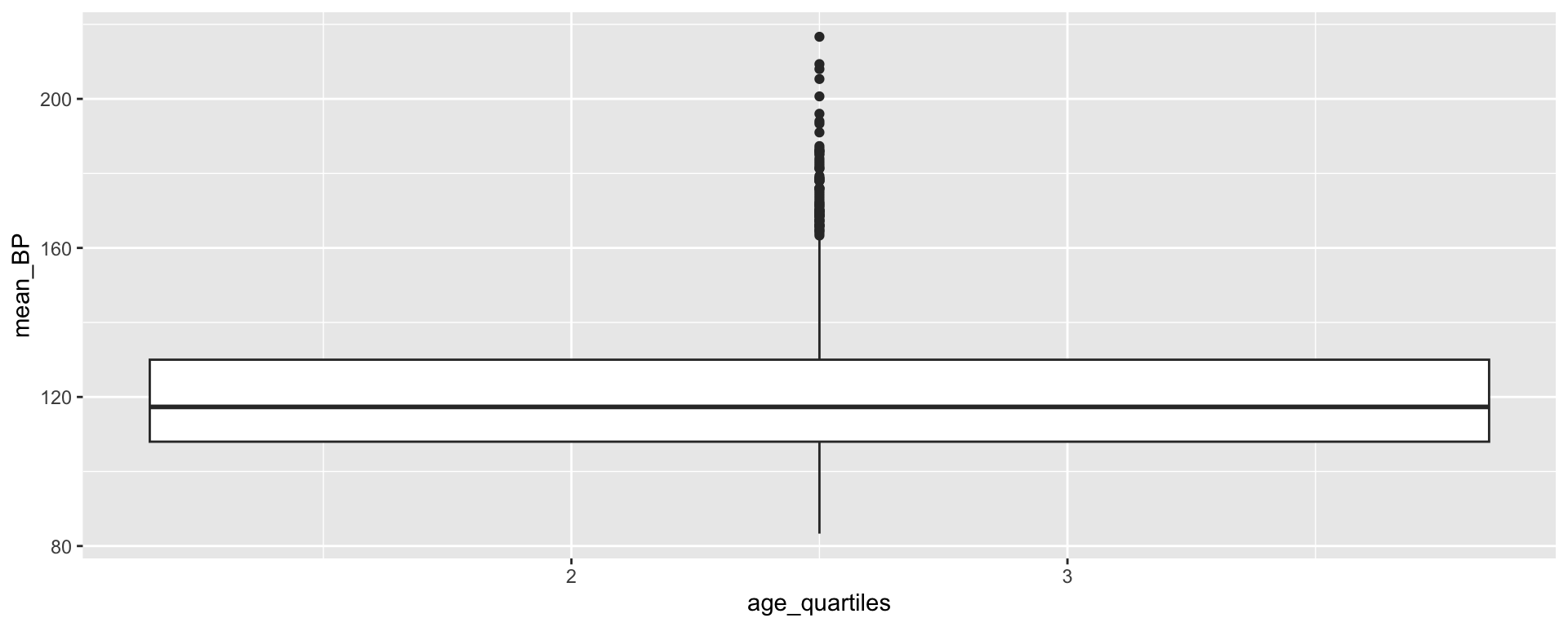
Transforming age_quartiles into a factor
[1] "factor"
Transforming age_quartiles into a factor
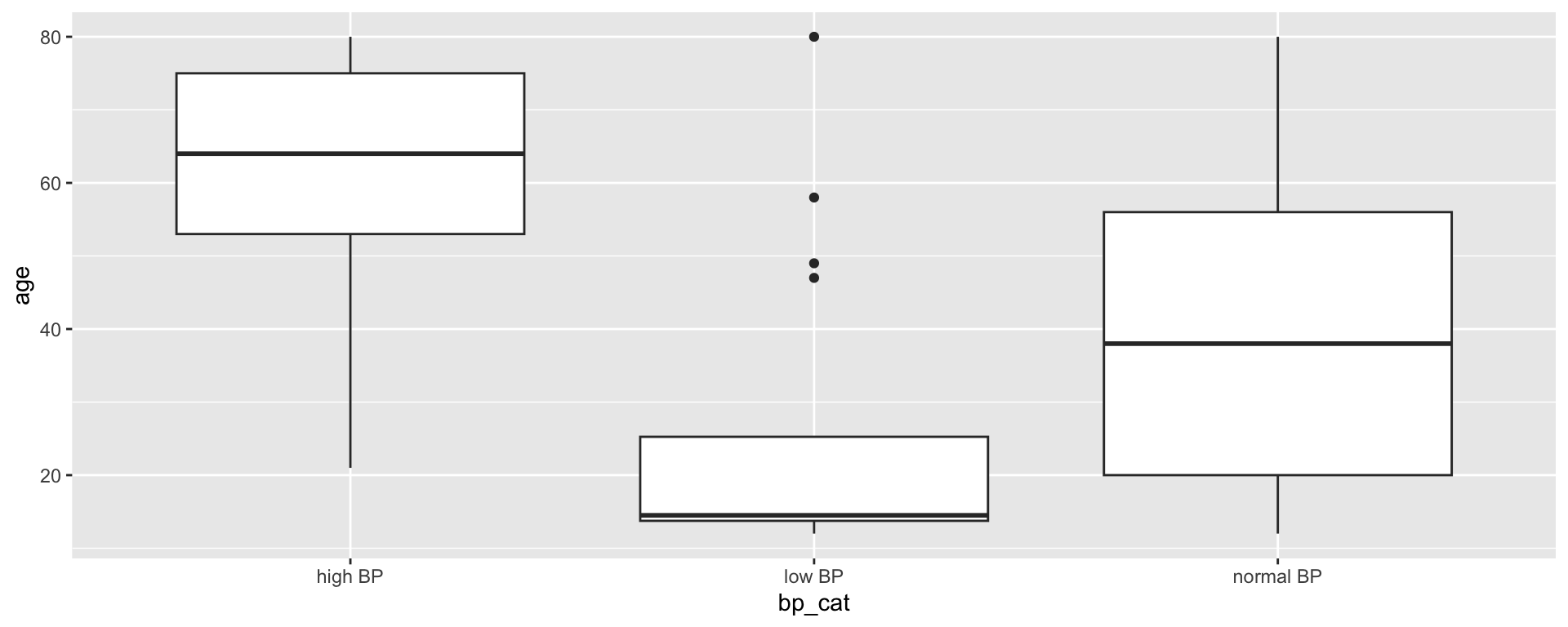
Creating blood pressure categories
Because bp_cat is not a factor yet, R has plotted the variable in alphabetical order by default. There may be some situations where this is sufficient, but for ordinal data, the order of the data is important!
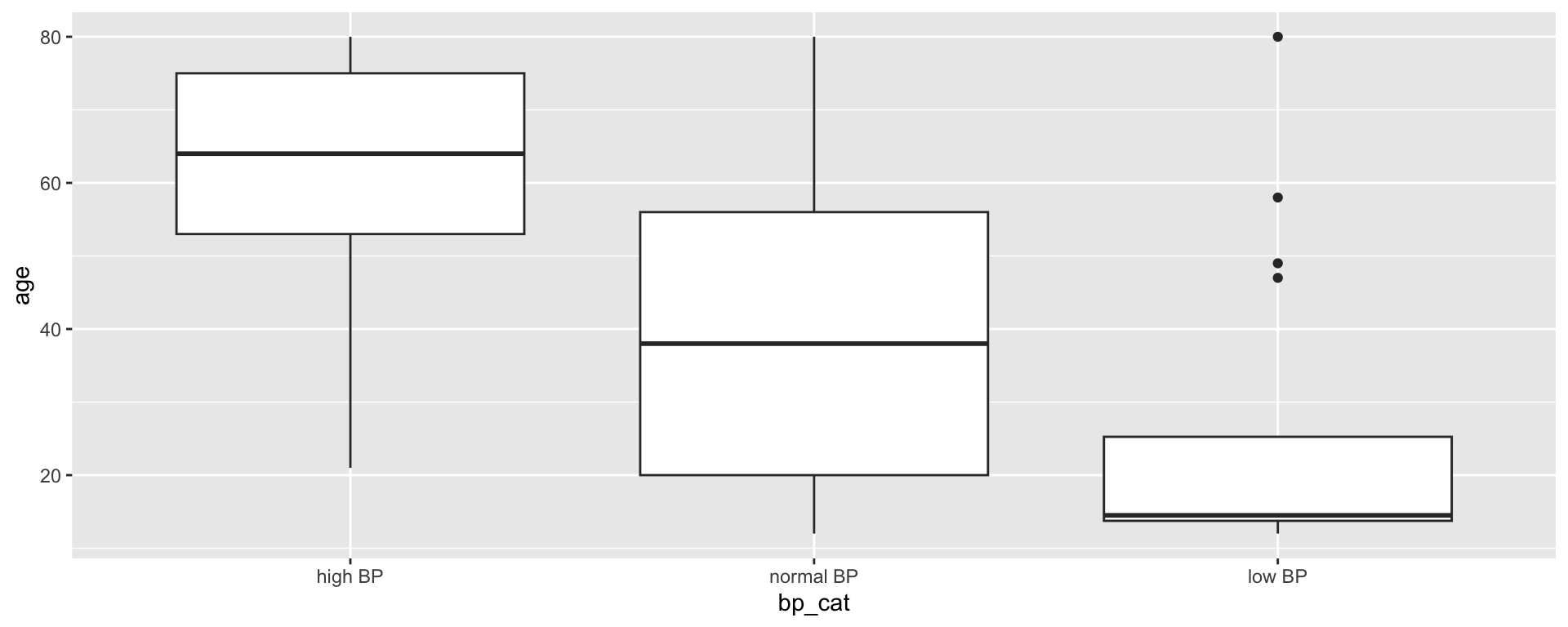
Transforming bp_cat into a factor
Working with Factors
The forcats:: package (short for “For Categorical”) is a helpful set of functions for working with factors.
![]()
Useful forcats:: functions
Check out the forcats:: cheatsheet for more info on how these functions work!
fct_drop()fct_relevel()fct_rev()fct_infreq()fct_inorder
![]()
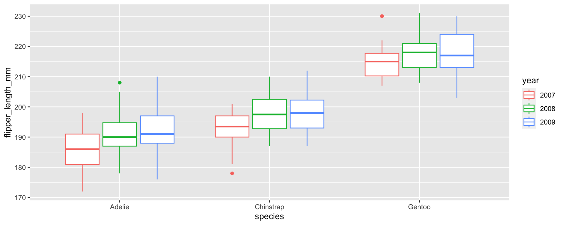
⚠️ Caution: factor → numeric
Let’s say we wanted to transform a “year” column from an integer to a factor to make a plot with a different boxplot for each year:
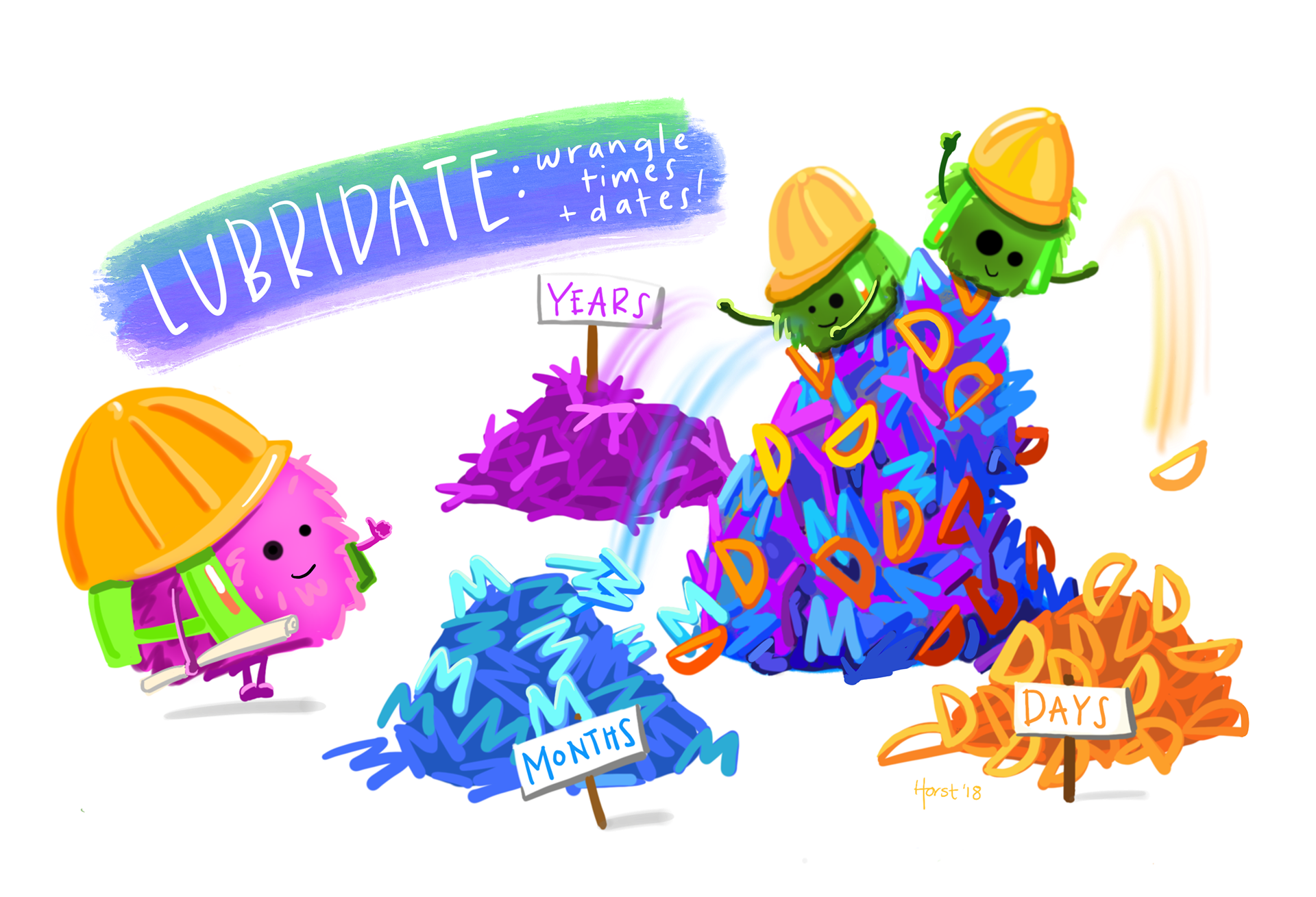
lubridate::
The lubridate:: package is a handy way of storing and processing date-time objects. lubridate:: categorizes date-time objects by the component of the date-time string they represent:
- year
- month
- day
- hour
- minute
- second
lubridate:: basics

Once you have a date-time object, you can use lubridate:: functions to extract and manipulate the different components.
lubridate:: basics
The function now() returns a date-time object, while today() returns just a date. lubridate:: also has functions that allow us to force the date into a date-time and the date-time into a date:
lubridate:: basics
With lubridate::, we can also work with dates as a whole, rather than their individual components. Let’s say we have a character string with the date, but we want R to transform it into a date-time object:
Time spans
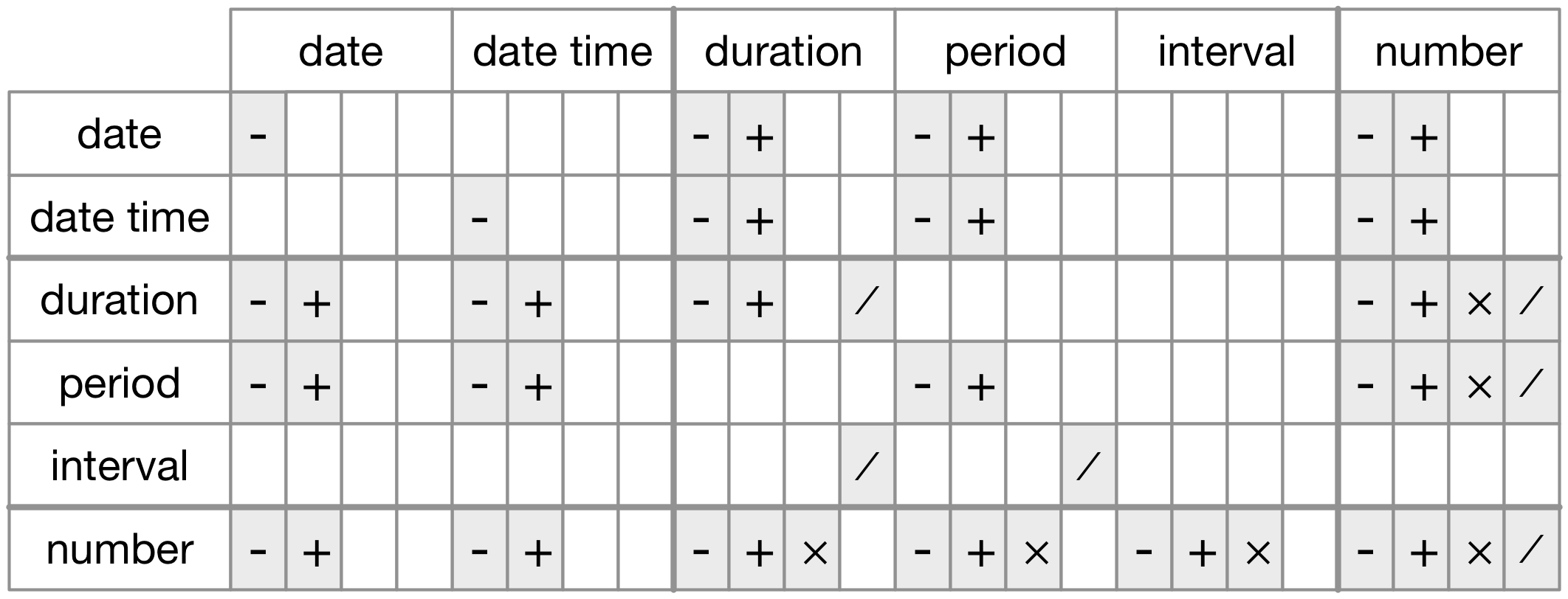
From R4DS Chapter 16: Dates and times

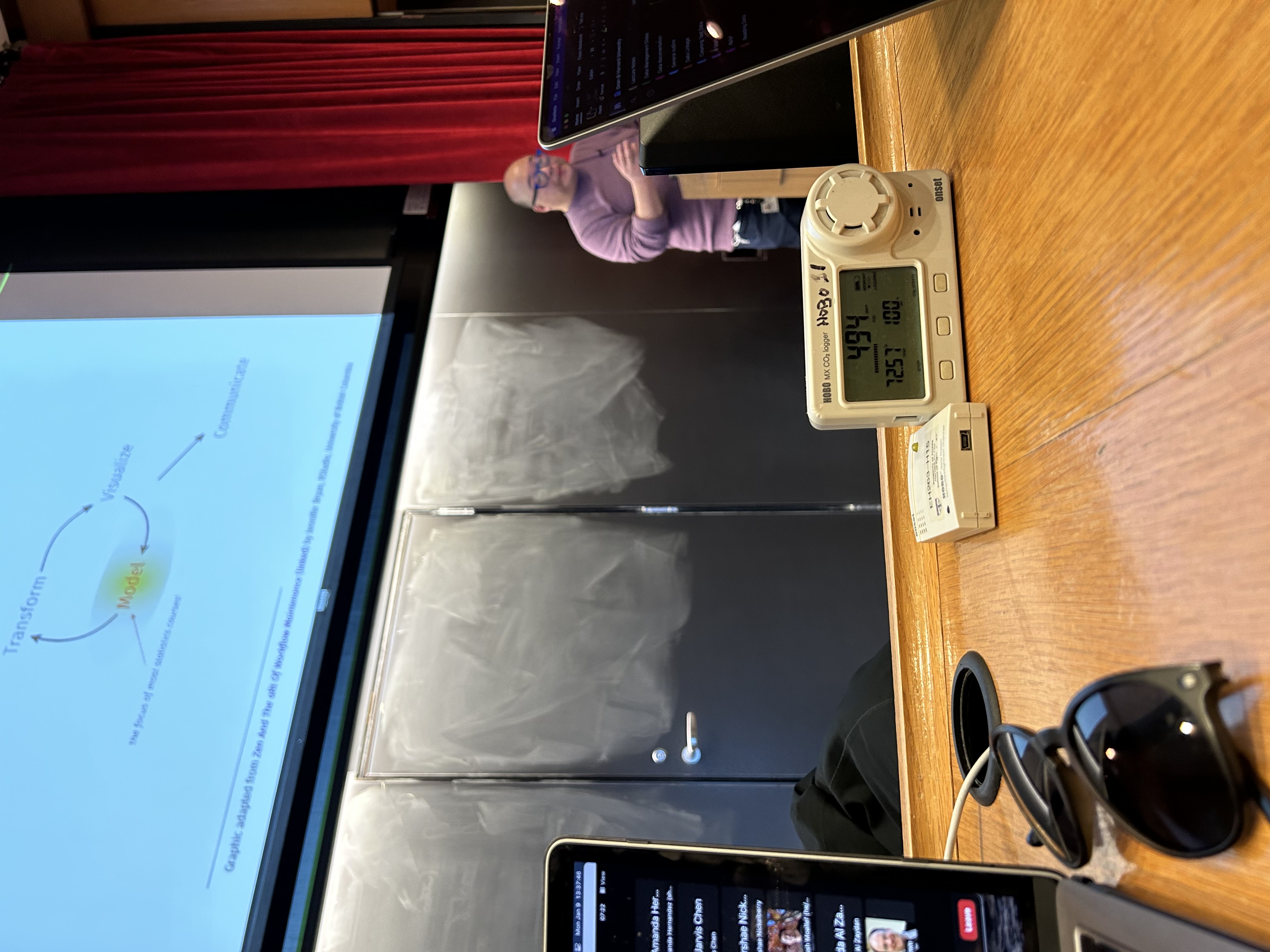
Example: Classroom CO\(_2\)
On the first day of ID529 in January 2023, I set up an instrument to log indoor temperature, relative humidity, and CO\(_2\) in G2.
The logger (called a HOBO) was set to collect data at 1-second intervals ~15 minutes before class began and ~15 minutes after class ended.
The data were cleaned and are now “long”
Example: Classroom CO\(_2\)
ggplot(hobo_g2_dt, aes(x = date_time, y = result))  +
  geom_line() +
  facet_wrap(~metric, scales = "free_y", ncol = 1) +
  scale_x_datetime(breaks = scales::date_breaks("30 mins"), date_labels = "%H:%M") +
  xlab("Time") +
  ylab("") +
  ggtitle(paste0("Indoor conditions in G2 (", unique(hobo_g2_dt$date), ")"))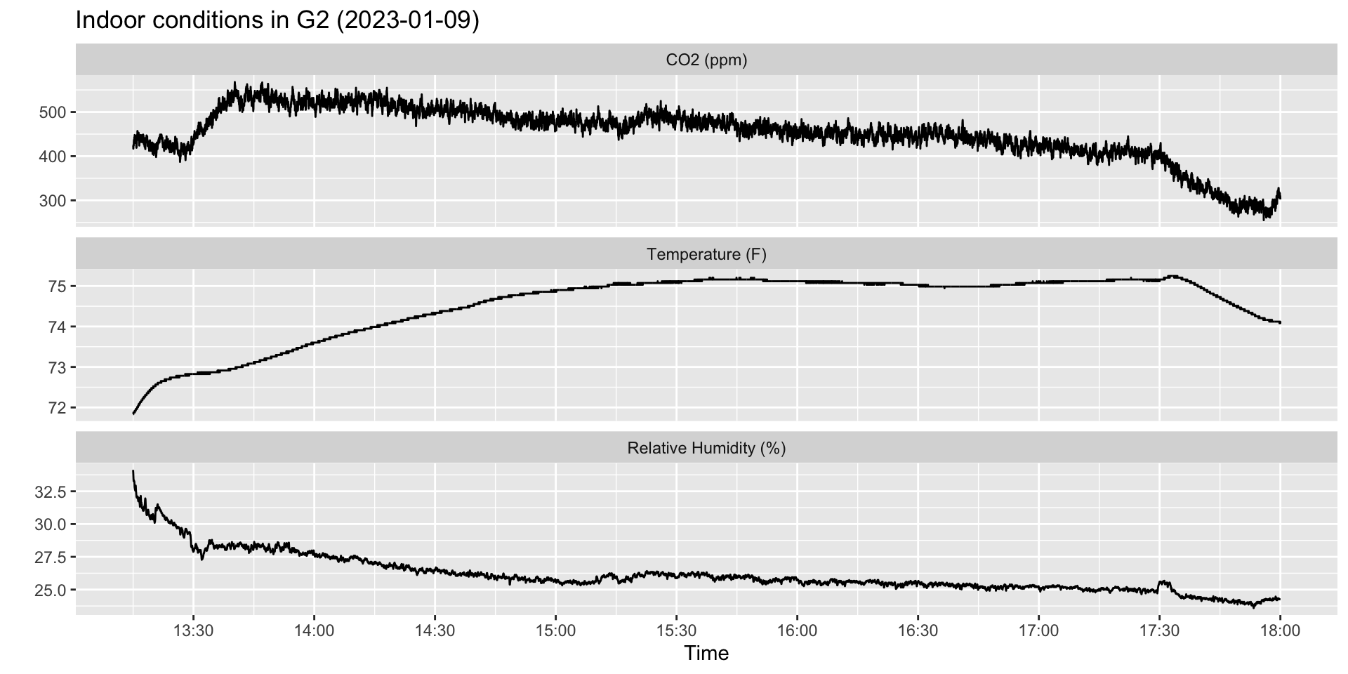
Example: Classroom CO\(_2\)
ggplot(hobo_g2_dt, aes(x = date_time, y = result))  +
  geom_line(color = "lightgrey", size = 1) +
  facet_wrap(~metric, scales = "free_y", ncol = 1) +
  theme_bw()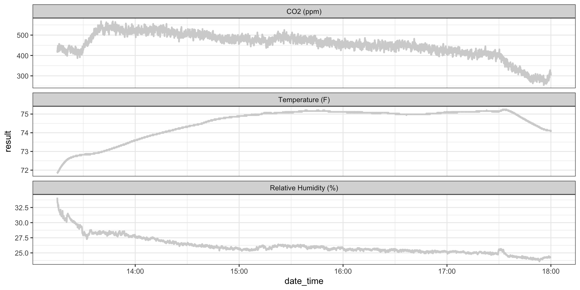
Example: Classroom CO\(_2\)
ggplot(hobo_g2_dt, aes(x = date_time, y = result))  +
  geom_line(color = "lightgrey", size = 1) +
  geom_line(hobo_g2_1min, mapping = aes(x = date_time, y = avg_1min), color = "slateblue3") +
  facet_wrap(~metric, scales = "free_y", ncol = 1) +
  theme_bw()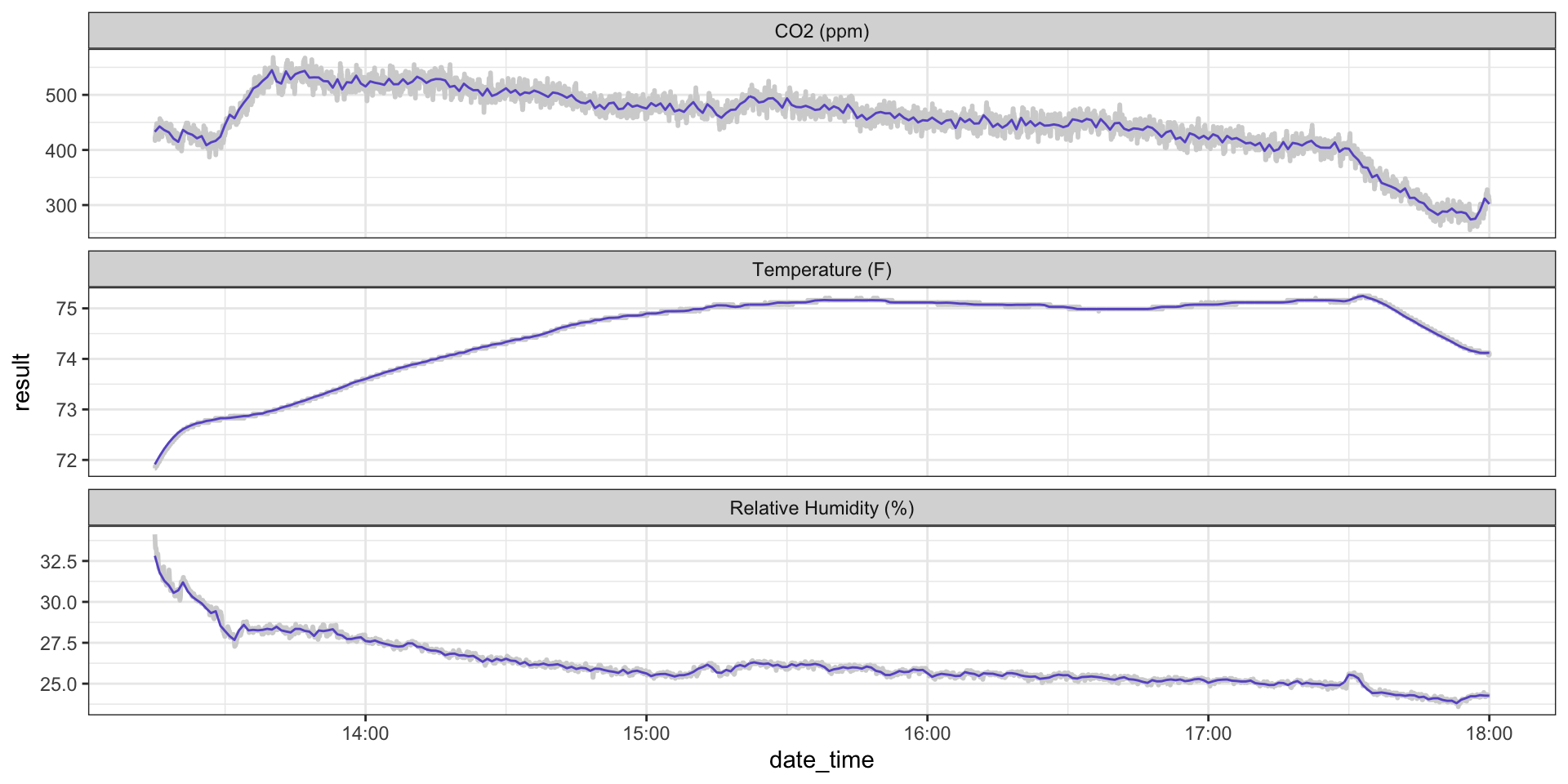
Example: Classroom CO\(_2\)
ggplot(hobo_g2_dt, aes(x = date_time, y = result))  +
  geom_line(color = "lightgrey", size = 1) +
  geom_line(hobo_g2_1min, mapping = aes(x = date_time, y = avg_1min), color = "slateblue3") +
  geom_line(hobo_g2_1hr, mapping = aes(x = date_time, y = avg_1hr), color = "paleturquoise2", alpha = 0.7) +
  facet_wrap(~metric, scales = "free_y", ncol = 1) +
  theme_bw()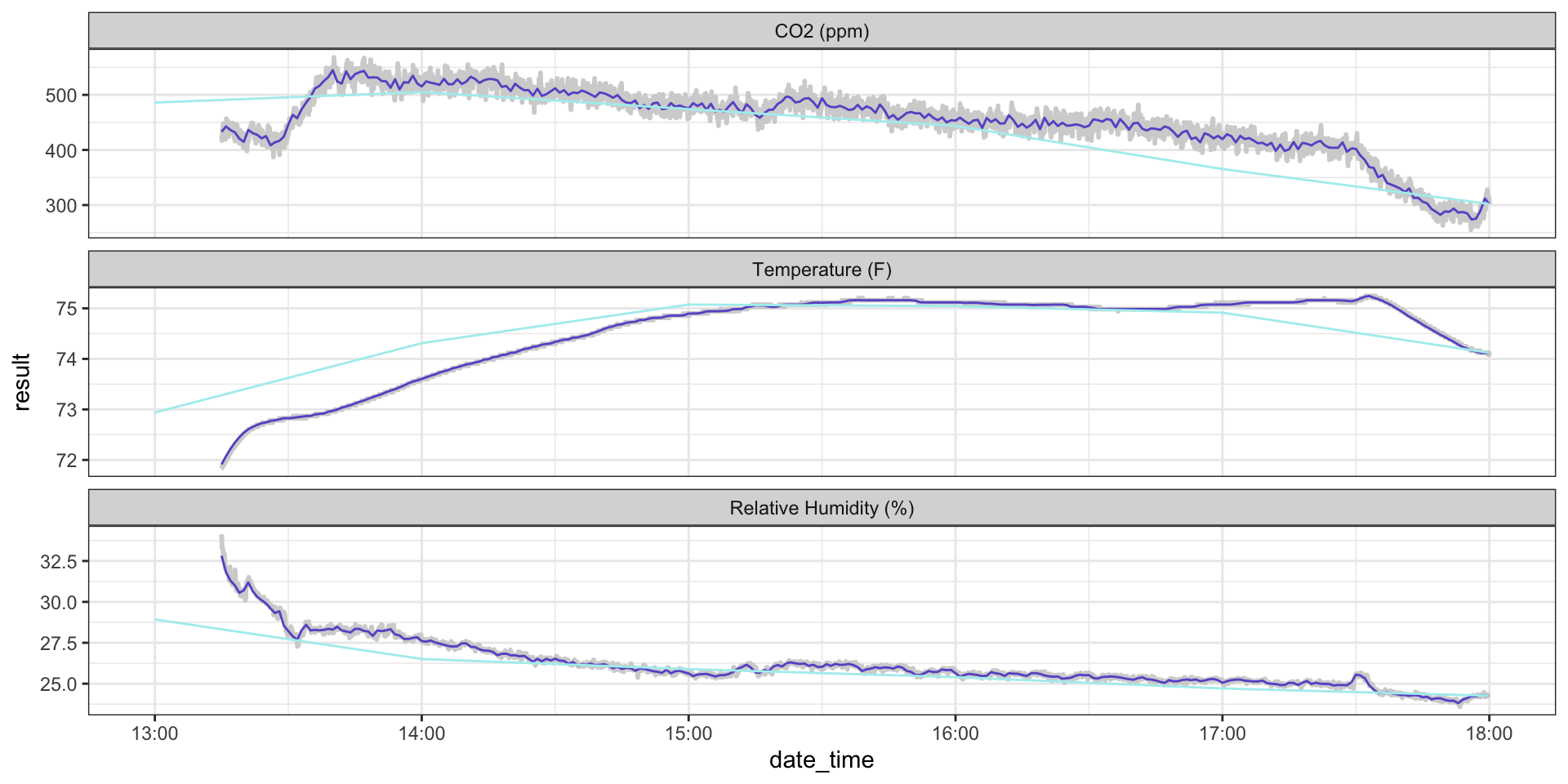
Example: Classroom CO\(_2\)
ggplot(hobo_g2_dt)  +
  geom_line(aes(x = date_time, y = result), color = "lightgrey", size = 1) +
  geom_line(hobo_g2_1min, mapping = aes(x = date_time, y = avg_1min), color = "slateblue3") +
  geom_line(hobo_g2_1hr, mapping = aes(x = date_time, y = avg_1hr), color = "paleturquoise2") +
  geom_rect(data = jan23_meeting_times %>%
              filter(dates %in% hobo_g2_dt$date),
              mapping = aes(xmin = start_datetime,
                            xmax = end_datetime,
                            ymin = 0, ymax = Inf),
              alpha = 0.2, fill = "lightpink") +
  facet_wrap(~metric, scales = "free_y", ncol = 1) +
  theme_bw()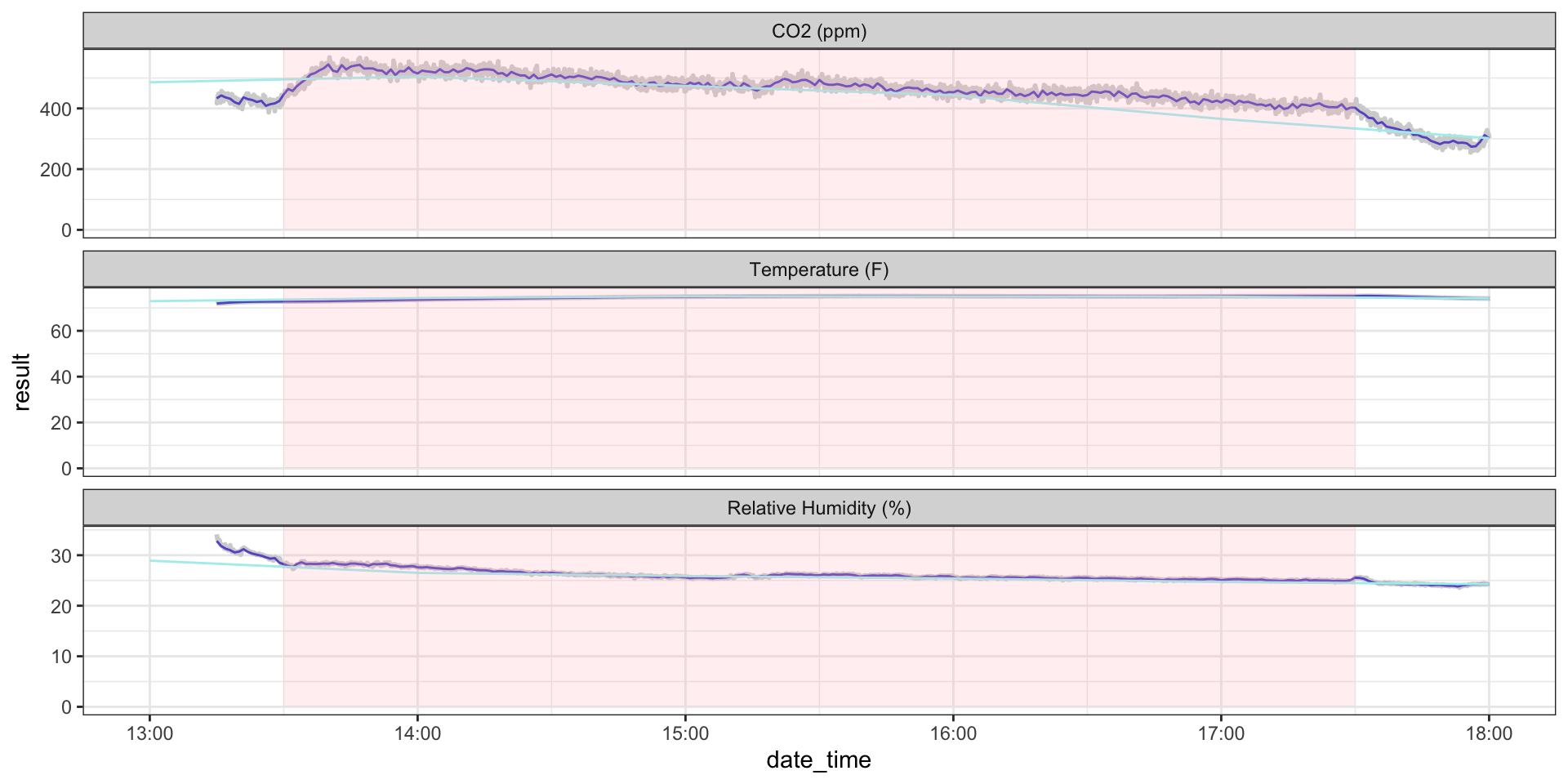
Example: COVID data
ggplot(
  covid_by_poverty_level |> filter(! is.na(poverty_cut)),
  aes(x = year_month,
      y = deaths_avg_per_100k,
      color = poverty_cut,
      group = poverty_cut)) +
  geom_line() +
  scale_color_brewer(palette = 'RdBu', direction = -1) +
  xlab("Date") +
  ylab("COVID-19 Mortality per 100k (monthly observations)") +
  ggtitle("Monthly County COVID-19 Mortality Estimates by Poverty Level in the US") +
  theme(axis.text.x = element_text(angle = 75, hjust = 1))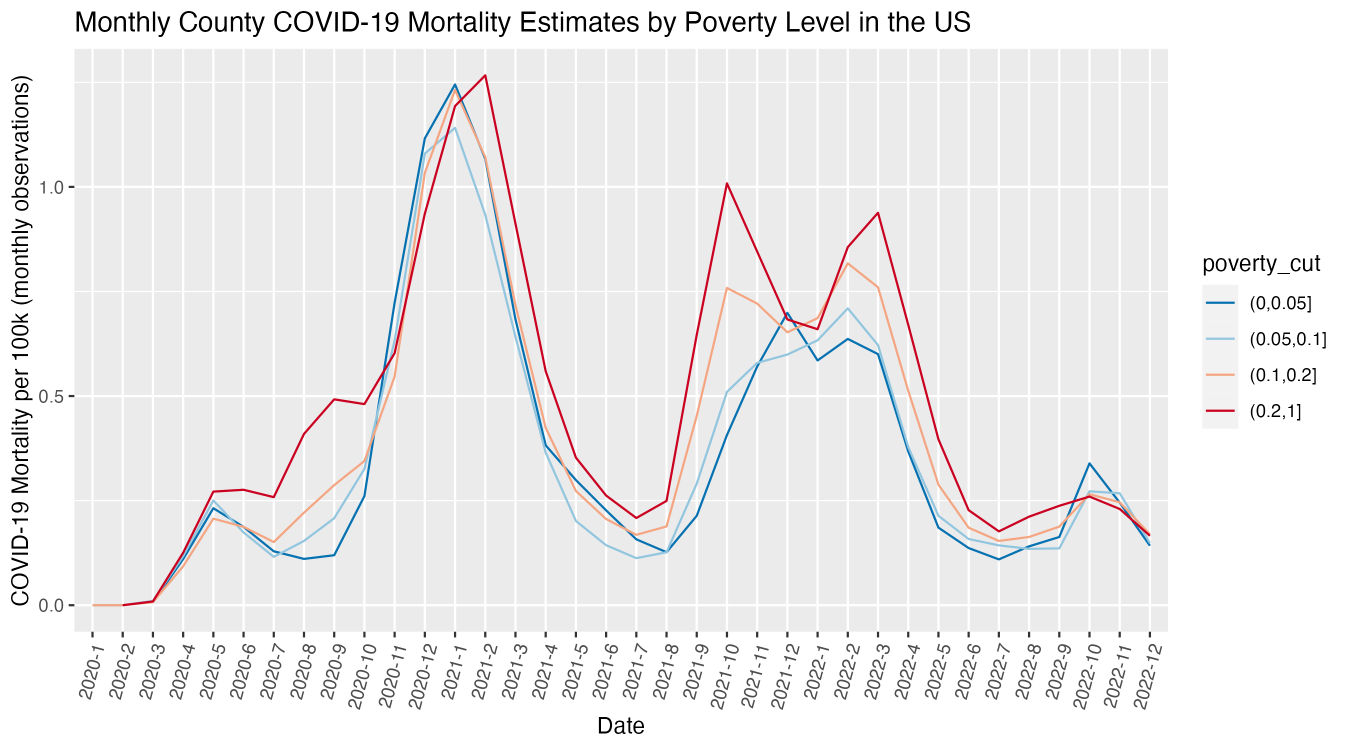
Key takeaways
Knowing how to manipulate factors and date-times can save you a ton of headache – you’ll have a lot more control over your data which can help with cleaning, analysis, and visualization!
forcats::andlubridate::give you a lot of the functionality you might needhms::is another package for working with times (stores time as seconds since 00:00:00, so you can easily convert between numeric and hms)
Factors and date-times can be tricky
Double check things are working as you expect along the way!!
If you can’t figure out why something isn’t working, take a break, and revisit it with fresh eyes.
There’s lots of documentation out there! The cheatsheets are great, as is The Epidemiologist R Handbook (https://epirhandbook.com/en/working-with-dates.html#working-with-dates-1)