id529_day5_regression_pretty

Follow along

`

https://bit.ly/id529_regression_models

Clone the repository and open it as a R Project in your RStudio.
Open the id529_day4_regression_models.R script. Run the data cleaning steps and fit the models on the df_completecase data frame

Some goals for today

Learn how to create some pretty tables
- Learn about the gtsummary package
- Learn about the sjPlot package
- Learn about the stargazer package
- Learn how to create plots of regression results

Data preparation

As we covered on Day 4, we begin by doing some data cleaning steps.

df <- NHANES  |>  
  # Remember that we have to restrict to people 25 and above
  filter(Age>=25)  |> 
  # recoding of the variables we're going to use
  mutate(agecat = case_when(
      Age < 35 ~ "25-34",
      35 <= Age & Age < 45 ~ "35-44",
      Age >= 45 & Age < 55 ~ "45-54",
      Age >= 55 & Age < 65 ~ "55-64",
      Age >= 65 & Age < 75 ~ "65-74",
      Age >= 75 ~ "75+"),
    # We want College Grad to be the reference category for education, so we'll
    # re-order the factor so that it is reversed from the way it came in the NHANES dataset
    Education = factor(Education, 
                       levels=rev(levels(NHANES$Education))),
    # Here we collapse Hispanic and Mexican into the Hispanic category
    racecat = factor(case_when(
      Race1 %in% c("Hispanic", "Mexican") ~ "Hispanic",
      Race1 %in% c("Asian", "Other") ~ "Other Non-Hispanic",
      Race1 == "Black" ~ "Black Non-Hispanic",
      Race1 == "White" ~ "White Non-Hispanic"), 
      levels = c("White Non-Hispanic", "Black Non-Hispanic", "Hispanic", "Other Non-Hispanic"))
  ) |>
  # select just variables we are going to use in the analysis
  select(ID, SurveyYr, Gender, Age, agecat, Education, racecat, BPSysAve, SmokeNow)

Restricting to non-missing observations

Though most regression functions will automatically drop observations with NA, sometimes we may want to explicitly filter out missing observations on any of the covariates we are going to include while model building to make sure that we can compare models based on the same number of observations.

df_completecase <- df |>
  filter(!is.na(BPSysAve) & !is.na(agecat) & !is.na(Gender) & !is.na(racecat))

Fitting multiple models

lm_model1 <- lm(BPSysAve ~ factor(Education), 
                data=df_completecase)
lm_model2 <- lm(BPSysAve ~ factor(Education) + factor(agecat) + Gender, 
                data=df_completecase)
lm_model3 <- lm(BPSysAve ~ factor(Education) + factor(agecat) + Gender + factor(racecat), 
                data=df_completecase)
lm_model4b <- lm(BPSysAve ~ factor(Education) + factor(agecat) + interaction(Gender,factor(racecat)), 
                 data=df_completecase)

Note that in lm_model4b I’ve used the interaction() function to create a categorical variable representing the cross-classified categories of gender and race/ethnicity

A workflow for extracting model results into tables

We have been emphasizing the idea of having a workflow that includes not only fitting a statistical model, but
- All of the data cleaning steps that help you get your data set up before you fit one or more statistical models
- All of the extraction and formatting steps that enable you to communicate the results after you fit your statistical model
Given that you will often have to refit models and tweak your analysis many times before presenting your final results, it is helpful to have a workflow that facilitates making edits or revisions and having these propagate to your final tables and figures

gtsummary package

The gtsummary package provides a user-friendly way to create publication-ready analytical and summary tables. It seamlessly integrates with the tidyverse and the gt package, allowing for easy manipulation and styling of tables. Some key functions in the gtsummary package include

tbl_summary(): Creates summary tables for descriptive statistics. It can automatically recognize and handle different data types (e.g., continuous, categorical) and present appropriate summary statistics.
tbl_regression(): Used for formatting regression model results. It takes a model object (like those from lm, glm, etc.) and returns a table of model estimates and statistics, making it easier to report regression analysis findings.
tbl_merge(): Allows for merging multiple gtsummary tables into a single table, which is useful for side-by-side comparisons.
tbl_stack(): Stacks multiple gtsummary tables vertically, which is helpful when you need to present similar tables for different groups or categories in a consolidated format.
add_p(): Adds p-values to the tables, which is particularly useful when summarizing statistical tests.

gtsummary: :tbl_regression( )

tbl_regression(lm_model1) |>
  bold_labels()

Characteristic	Beta	95% CI¹	p-value
factor(Education)
College Grad	—	—
Some College	3.8	2.7, 4.8	<0.001
High School	5.1	3.9, 6.4	<0.001
9 - 11th Grade	4.7	3.3, 6.1	<0.001
8th Grade	7.9	6.1, 9.8	<0.001
¹ CI = Confidence Interval

gtsummary: :tbl_regression( )

I don’t like that the table has the label “factor(Education)”, so I can modify this using the label= argument

tbl_lm_model1 <- 
  tbl_regression(lm_model1, label = list('factor(Education)' ~ 'Education')) |>
  bold_labels() 
tbl_lm_model1

Characteristic	Beta	95% CI¹	p-value
Education
College Grad	—	—
Some College	3.8	2.7, 4.8	<0.001
High School	5.1	3.9, 6.4	<0.001
9 - 11th Grade	4.7	3.3, 6.1	<0.001
8th Grade	7.9	6.1, 9.8	<0.001
¹ CI = Confidence Interval

gtsummary: :tbl_regression( )

Note that we can add model fit statistics using add_glance_table()

tbl_lm_model1_glance <- 
  tbl_regression(lm_model1, label = list('factor(Education)' ~ 'Education')) |>
  bold_labels() |> 
  add_glance_table()
tbl_lm_model1_glance

Characteristic	Beta	95% CI¹	p-value
Education
College Grad	—	—
Some College	3.8	2.7, 4.8	<0.001
High School	5.1	3.9, 6.4	<0.001
9 - 11th Grade	4.7	3.3, 6.1	<0.001
8th Grade	7.9	6.1, 9.8	<0.001
R²	0.019
Adjusted R²	0.018
Sigma	17.3
Statistic	30.4
p-value	<0.001
df	4
Log-likelihood	-26,991
AIC	53,994
BIC	54,035
Deviance	1,886,669
Residual df	6,319
No. Obs.	6,324
¹ CI = Confidence Interval

set_gtsummary_theme

gtsummary has a number of themes that allow us to format the tables for different journals
Some available formats are:
- theme_jama()
- theme_lancet()
- theme_bmj()
- theme_annals()
Here we format to the JAMA journal format

set_gtsummary_theme(theme_gtsummary_journal("jama"))

Compare model results

We might want to combinete several different model results into a single table.
First we format each of the models using tbl_regression()

# Note for this first one that I am showing how to integrate this
# into a workflow where you start with the analytic data frame,
# pipe it into lm() and then pipe the results into
# tbl_regression.
# BUT: note that the first pipe has to be the magrittr pipe %>%
# and not the "new" pipe |>
tbl_lm_model1 <- df_completecase %>%
  lm(BPSysAve ~ factor(Education), 
     data=.) |>
  tbl_regression(intercept=TRUE,
                 label = list('factor(Education)' ~ 'Education'))

Compare model results

tbl_lm_model2 <- lm_model2 |> 
  tbl_regression(intercept=TRUE,
                 label = list('factor(Education)' ~ 'Education',
                              'factor(agecat)' ~ 'Age category'))

tbl_lm_model3 <- lm_model3 |>
  tbl_regression(intercept=TRUE,
                 label = list('factor(Education)' ~ 'Education',
                              'factor(agecat)' ~ 'Age category',
                              'factor(racecat)' ~ 'Racialized group'))

tbl_lm_model4 <- lm_model4b |>
  tbl_regression(intercept=TRUE,
         label = list('factor(Education)' ~ 'Education',
                      'factor(agecat)' ~ 'Age category',
                      'interaction(Gender, factor(racecat))' ~ 'Gender X Racialized group'),
                 )

Compare model results

Now that each of the models has been formatted, I can use tbl_merge to put the models together to be shown side-by-side

tbl_merge_ex1 <-
  tbl_merge(
    tbls = list(tbl_lm_model1,
                tbl_lm_model2,
                tbl_lm_model3,
                tbl_lm_model4),
    # the tab_spanner argument specifies the headings at the top of the table
    # that span multiple columns
    tab_spanner = c("**Model 1**", "**Model 2**", "**Model 3**", "**Model 4**")
  )

Compare model results

tbl_merge_ex1

Characteristic	Model 1		Model 2		Model 3		Model 4
Characteristic	Beta (95% CI)¹	p-value	Beta (95% CI)¹	p-value	Beta (95% CI)¹	p-value	Beta (95% CI)¹	p-value
(Intercept)	119 (118 to 119)	<0.001	109 (108 to 110)	<0.001	109 (108 to 110)	<0.001	109 (108 to 110)	<0.001
Education
College Grad	—		—		—		—
Some College	3.8 (2.7 to 4.8)	<0.001	3.2 (2.2 to 4.2)	<0.001	2.9 (1.9 to 3.9)	<0.001	2.9 (1.9 to 3.9)	<0.001
High School	5.1 (3.9 to 6.4)	<0.001	3.9 (2.7 to 5.0)	<0.001	3.4 (2.3 to 4.5)	<0.001	3.4 (2.3 to 4.5)	<0.001
9 - 11th Grade	4.7 (3.3 to 6.1)	<0.001	3.2 (1.9 to 4.5)	<0.001	2.7 (1.3 to 4.0)	<0.001	2.7 (1.3 to 4.0)	<0.001
8th Grade	7.9 (6.1 to 9.8)	<0.001	3.7 (1.9 to 5.4)	<0.001	3.6 (1.8 to 5.5)	<0.001	3.7 (1.9 to 5.5)	<0.001
Age category
25-34			—		—		—
35-44			4.0 (2.8 to 5.2)	<0.001	4.1 (2.9 to 5.3)	<0.001	4.1 (2.8 to 5.3)	<0.001
45-54			6.7 (5.5 to 7.9)	<0.001	6.7 (5.5 to 7.9)	<0.001	6.6 (5.4 to 7.8)	<0.001
55-64			13 (11 to 14)	<0.001	13 (11 to 14)	<0.001	13 (11 to 14)	<0.001
65-74			16 (14 to 17)	<0.001	16 (14 to 17)	<0.001	16 (14 to 17)	<0.001
75+			24 (22 to 25)	<0.001	24 (22 to 25)	<0.001	24 (22 to 25)	<0.001
Gender
female			—		—
male			4.0 (3.2 to 4.8)	<0.001	4.1 (3.3 to 4.8)	<0.001
Racialized group
White Non-Hispanic					—
Black Non-Hispanic					4.4 (3.1 to 5.7)	<0.001
Hispanic					0.03 (-1.2 to 1.3)	0.96
Other Non-Hispanic					-1.3 (-2.8 to 0.24)	0.10
Gender X Racialized group
female.White Non-Hispanic							—
male.White Non-Hispanic							3.7 (2.8 to 4.6)	<0.001
female.Black Non-Hispanic							4.8 (3.0 to 6.6)	<0.001
male.Black Non-Hispanic							7.7 (5.9 to 9.6)	<0.001
female.Hispanic							-0.72 (-2.5 to 1.1)	0.43
male.Hispanic							4.4 (2.7 to 6.1)	<0.001
female.Other Non-Hispanic							-3.0 (-5.1 to -0.92)	0.005
male.Other Non-Hispanic							4.3 (2.1 to 6.5)	<0.001
¹ CI = Confidence Interval

Output options

In addition to embedding in a RMarkdown or Quarto file, we can also output directly to an html file

# We can save this as html
tbl_merge_ex1 %>%
  as_gt() %>%
  gt::gtsave(filename = "lm_models.html")

We can save to a Word file (docx)

# We can save this as a Word file (docx)
tbl_merge_ex1 %>%
  as_flex_table() %>%
  flextable::save_as_docx(path="lm_models.docx")

We can save to an Excel file

# We can even be fancy and export to an Excel file
tbl_merge_ex1 %>%
  as_hux_xlsx(file="lm_models.xlsx")

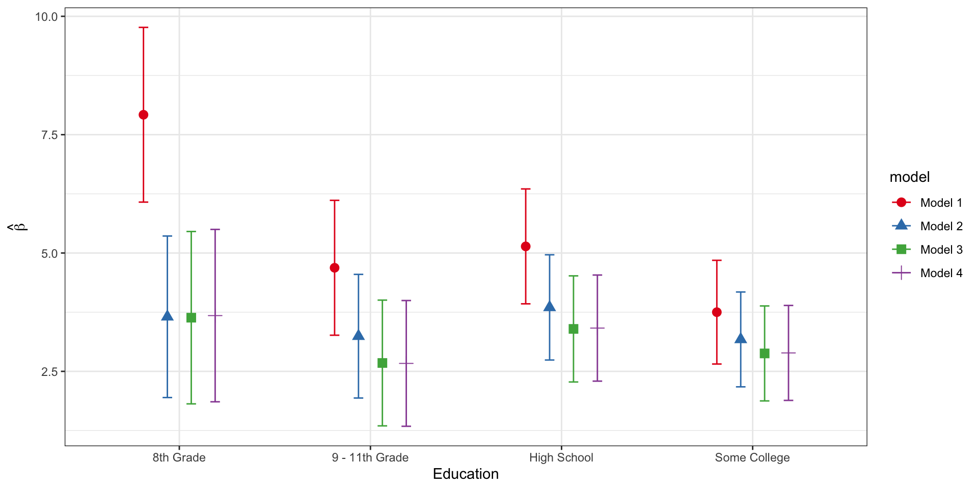
A workflow for plotting model estimates

Let’s say that we want to compare estimates of the education effect in the crude and adjusted models.
Here, I show an example of using broom::tidy to
- extract the model estimates,
- stack them together in a tibble,
- filter out just the education terms,
- and pipe the tibble into ggplot in order to plot the estimates.

.{smaller}

# Extract the education effects from each model and combine in a tibble
lm_education_estimates <- bind_rows(broom::tidy(lm_model1, conf.int=TRUE) %>% 
                                      mutate(model = "Model 1"),
                                    broom::tidy(lm_model2, conf.int=TRUE) %>%
                                      mutate(model = "Model 2"),
                                    broom::tidy(lm_model3, conf.int=TRUE) %>% 
                                      mutate(model = "Model 3"),
                                    broom::tidy(lm_model4b, conf.int=TRUE) %>%
                                      mutate(model = "Model 4")) %>%
  # here, we use stringr::str_detect to detect the entries
  # where term includes the string 'Education'
  filter(stringr::str_detect(term, "Education")) %>%
  # here, we use the separate() function to pull out the category labels
  # from term so that we can have nice labeling in the plot
  separate(col=term, sep=17, into=c("term", "category"), convert=TRUE)

# Use ggplot to plot the point estimates and 95% CIs
# Note that we are differentiating the models by color AND by the shape of the plotting symbol
ggplot(lm_education_estimates, aes(x=category, y=estimate, color=model, shape=model)) +
  # position=position_dodge() is specified so that the estimates are side by side rather than
  # plotted on top of one another
    geom_point(position=position_dodge(0.5), size=3) +
  # geom_errorbar allows us to plot the 95% confidence limits
    geom_errorbar(aes(ymin=conf.low, ymax=conf.high), position=position_dodge(0.5), width=0.2) +
  # scale_color_brewer allows me to control the colors for plotting the different models
    scale_color_brewer(palette="Set1") +
    labs(x="Education", y=expression(hat(beta))) +
    theme_bw()

Regression modeling workflows: making it pretty

Follow along

Some goals for today

Data preparation

Restricting to non-missing observations

Fitting multiple models

A workflow for extracting model results into tables

gtsummary package

gtsummary: :tbl_regression( )

gtsummary: :tbl_regression( )

gtsummary: :tbl_regression( )

set_gtsummary_theme

Compare model results

Compare model results

Compare model results

Compare model results

Output options

A workflow for plotting model estimates

.{smaller}