Introduction to R Markdown

ID 529: Data Management and Analytic Workflows in R

Dean Marengi | Tuesday, January 16th, 2024

Learning objectives


  • Understand the advantages of R Markdown (and Quarto) as tools for reproducible research
  • Learn about the basic components that make up R Markdown documents
    • YAML headers
    • Plain text
    • Code chunks
  • Learn how to use R Markdown to generate reproducible reports
    • Integrating different elements of a typical report including descriptive text, analysis results and visualizations, inline quantitative statements
    • Organizing and formatting R Markdown files for research collaboration
    • Exporting reports to different output formats (e.g., .html, .docx, .pdf and more)

R Markdown Example Available on GitHub


  • Simple Example: https://github.com/dmarengi/sample-rmd
    • Create a copy of the repository on your local computer
      • Clone the repository to your local device
      • Alternatively, Click <> Code > Download Zip


Background

First, a little about Markdown

  • Markdown is a markup language used to format plain text documents (it’s not unique to R)
    • Uses a simple, human-readable syntax to apply formatting
    • Contrasts with other common tools used for text formatting (e.g., Microsoft Word documents)
      • Formatting appears simple, but is complicated ‘under the hood’
    • Widely used, and allows for easy conversion to different file types (e.g., PDFs, html files, etc.)


  • Markdown can be used to generate:
    • Reports (as we’ll discuss)
    • Books
    • Slides
    • Websites
    • And more!


# Markdown: a love story

There's a beauty in the *simplicity* of formatting text with `Markdown`! It's capable of giving so much, ***while asking for so little***. Not like those text formatting tools from "**Big Word Processor,**" with all of their fancy bells and whistles.
    
## What's great about Markdown, you ask?

- It's easy to read and write
- It's platform-agnostic
    - No specific software required
    - Highly compatiable with a range of tools
- Overall, less fuss!


Rendered output on the next slide!


Markdown: A love story

There’s a beauty in the simplicity of formatting text with Markdown! It’s capable of giving so much, while asking for so little. Not like those text formatting tools from “Big Word Processor”, with all of their fancy bells and whistles.


What’s great about Markdown, you ask?

  • It’s easy to read and write
  • It’s platform-agnostic
    • No specific software required
    • Highly compatible with a range of tools
  • Overall, less fuss!

So, what is R Markdown?

  • R Markdown is an extension of Markdown
  • Integrates with the R Studio IDE
  • Allows R users to combine into one document:
    • Markdown formatted text
    • R code chunks
    • Analysis results and visualizations
    • Mathematical expressions
  • “knit” documents to different output formats (HTML files, PDFs, Word Documents, etc.)
# Install R Markdown (if you have not already done so)
install.packages("rmarkdown")

Great tool for promoting transparency and reproducible research, as it allows researchers to easily consolidate their code, results, and interpretations into a single document!

R Markdown vs. Quarto

  • R Markdown is optimized for use with R and R Studio
  • Unlike R Markdown, Quarto does not require R
    • Can be used with other programming languages (e.g., Python, Javascript, etc.)


  • Quarto unifies the functionality of the R Markdown package ecosystem (rmarkdown, bookdown, etc.) into a single technical publishing system
  • Can use either, but Quarto will continue to be updated with new features and functionality
    • Can render existing .Rmd files as .qmd files

R Markdown Components

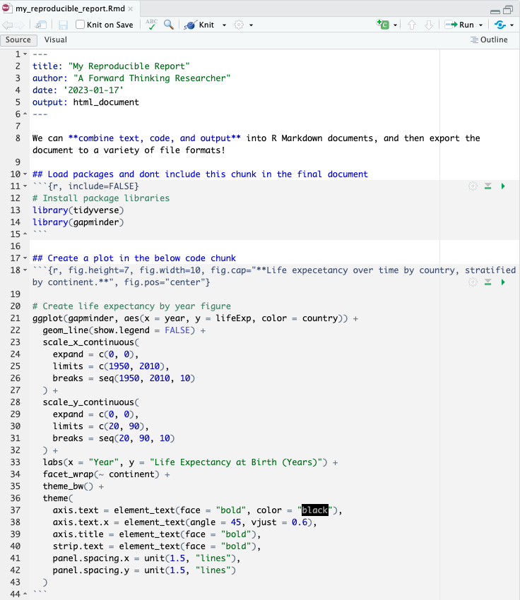
The Components of R Markdown Documents

  • R Markdown files (.Rmd) are plain text files designed to contain three types of content:
    • Plain text for narrative
    • Code chunks
    • Metadata to inform how the file is rendered and exported (YAML Header)
  • Code chunks
    • Delimited by ```{r} and ```
  • YAML header
    • Section included at the top of the .Rmd file
    • Metadata delimited by --- and ---
  • Plain text
    • Written throughout the document
    • Markdown used to apply text formatting

YAML Header


---
title:  "Reproducible Research"
author: "A prudent researcher"
date:   "2024-01-16"
output: html_document
---
  • The YAML header is used to customize the R Markdown document
  • Takes key-value pairs to specify document options and settings
    • E.g., title, author, date, output format, document class or other parameters
    • For HTML files, a CSS style sheet may also be referenced in the YAML Header
    • YAML header information is used to configure behavior of the ‘R Markdown engine’ to convert documents into a final output format

YAML Header: Some output formats

---
title:  "Reproducible Research"
author: "A prudent researcher"
date:   "2024-01-16"
output: 
  pdf_document: default
  html_document: default
  word_document: default
  github_document: default
---
  • Output formats for the .Rmd file can be specified in the YAML header
  • In the above example, we can knit our Rmd file into any of the specified formats (pdf, html, or docx)
  • Note that the indentation is meaningful for YAML headers!
    • Indentation creates a hierarchy and structure for YAML header information
    • Incorrect indentation will cause the YAML parser to fail when rendering the .Rmd file

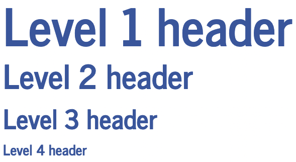
Markdown syntax: Headings


Markdown text

# Level 1 header

## Level 2 header

### Level 3 header

#### Level 4 header

Rendered text

Markdown syntax: Basic text formatting


Markdown text

*italics* or _italics_


**bold** or __bold__        


***bold and italic*** or 
___bold and italic___    

~~strikethrough~~

superscripts^2^

Rendered text

italics or italics

bold or bold

bold and italic or
bold and italic

strikethrough

superscripts2

Markdown syntax: Lists


Markdown text

- item 1
- item 2
- item 3
  - item 3.1
  - item 3.2
    - item 3.2.1


1. item 1
2. item 2
3. item 3
  - item 3.1
  - item 3.2
    - item 3.2.1

Rendered text

  • item 1
  • item 2
  • item 3
    • item 3.1
    • item 3.2
      • item 3.2.1
  1. item 1
  2. item 2
  3. item 3
    • item 3.1
    • item 3.2
      • item 3.2.1

Markdown syntax: Lists (alternative)


Markdown text

* item 1
* item 2
* item 3
  + item 3.1
  + item 3.2
    + item 3.2.1


1. item 1
2. item 2
3. item 3
  + item 3.1
  + item 3.2
    + item 3.2.1

Rendered text

  • item 1
  • item 2
  • item 3
    • item 3.1
    • item 3.2
      • item 3.2.1
  1. item 1
  2. item 2
  3. item 3
    • item 3.1
    • item 3.2
      • item 3.2.1

Markdown syntax: Blockquotes


Markdown text

> "Block quotes are neat."
> 
> -- Hodu

Rendered text

“Block quotes are neat.”

– Hodu

Markdown syntax: Embedding Images


Images from file storage

![](images/hex-rmarkdown.png)


Images from web sources

![](https://i0.wp.com/johnmackintosh.net/assets/img/blog/20220921-padme.jpeg)

Code chunks


  • Code chunks can be inserted throughout the R Markdown document
  • To insert a code chunk click the green code chunk button in the top right corner of .Rmd document
    • Alternatively, use a keyboard shortcut!
    • Mac: command + option + i
    • PC: control + alt + i
  • All code chunks are run, in the order they appear, when the file is rendered
```{r}
# This is a code chunk! 
print("Add code here, just like you would in an R script")
```
```{r}
print("Code chunks are run in order when the file renders")
```
```{r}
print("So, be sure to organize your code accordingly!")
```

Code chunks: Chunk options


  • Output from each code chunk can be customized
  • Set using knitr chunk options
    • Included between the curly braces {r ...}
  • A few commonly used options include:
    • include = FALSE: Exclude chunk code/output
    • echo = FALSE: Show code output, but not the code
    • warning = FALSE: Don’t include warning messages
    • fig.height = ...: Set output figure height (in.)
    • fig.width = ...: Set output figure width (in.)

See the resources linked below for more; there are a lot!

```{r, echo = TRUE, warning = FALSE}
# Show the code and output in rendered file
```
```{r, fig.height = 3, fig.width = 5}
# Set the output figure height and width
ggplot(data, aes(x = var1, y = var2)) +
  geom_point()
```

Code chunks: Global options


  • Instead of setting chunk options for each code chunk, you can alternatively set global chunk options
    • That is, you can apply a configuration or option across all code chunks in the Rmd document
    • Global settings can be overridden by setting options on individual code chunks
```{r, knitr::opts_chunk$set(echo=FALSE)}
# This knitr option sets echo=FALSE as a global option
# All code chunks will therefore omit code from the rendred output file
```

A note on LaTeX


Note: If you want to create pdf reports, you will need to install a LaTeX distribution. For R, it’s recommended that the TinyTex distribution be used. To do this, you can install the tinytex R package. Check out the resources linked below for more details.


install.packages("tinytex")
tinytex::install_tinytex()

# to uninstall TinyTeX, run tinytex::uninstall_tinytex() 

Embedding Mathematical Expressions

  • Within R Markdown files, you can also incorporate mathematical expressions
  • Uses LaTeX syntax
    • Expressions wrapped in single dollar signs $..$ are displayed “in-line”
    • Expressions wrapped in double dollar signs $$..$$ render as stand-alone equations
  • The syntax can be confusing at first, but will make sense the more you use it!
$$
\begin{equation}
\hat{Y}_i = \hat{\beta}_0 + \hat{\beta}_1 X_i + \hat{\epsilon}_i
\end{equation}
$$
This is some text with an in-line expressions like $\hat{Y}_i$ and $\hat{\beta}_1 X_i$. Pretty cool, right?


\[ \begin{equation} \hat{Y}_i = \hat{\beta}_0 + \hat{\beta}_1 X_i + \hat{\epsilon}_i \end{equation} \] This is some text with an in-line expressions like \(\hat{Y}_i\) and \(\hat{\beta}_1 X_i\). Pretty cool, right?

Let’s look at an Rmd file in R Studio!

Resources

Introductory Information

Resources to quickly reference

More comprehensive resources