[1] "species"           "island"            "bill_length_mm"
[4] "bill_depth_mm"     "flipper_length_mm" "body_mass_g"
[7] "sex" "year" Factors and date-times
ID 529: Data Management and Analytic Workflows in R
Jarvis Chen
thanks to Amanda Hernandez for the original version of this presentation!
Thursday, January 15th, 2026
15 Jan 2026
01-15-26
2026-01-15
as_date(44575, origin = “1904-01-01”)
Follow along
Learning objectives
Understand the importance of properly handling factors and date-times in data analysis
Learn about challenges and common mistakes when working with factors and date-times in R
Be familiar with packages for working with factors and date-times
forcats::for manipulating factors in Rlubridate::for handling date-times
Factors
What are factors?
A factor is an integer vector that uses levels to store attribute information.
- Levels serve as the logical link between integers and categorical values.
Factors retain the order of your variables through levels.
Factors have a lot more rules than character strings
- Once you understand the rules, you have a lot more manual control over your data (while still being reproducible)
What are factors?
Factors are particularly useful for ordinal data , where our data is categorical, but there is an order to the categories.
Factors are also useful when values are repeated frequently, and there’s a pre-specified set of distinct levels.
For example:
Age groups
Quantile groups
Months/Days of the week
Working with factors
Your data may already have variables as factors, or you can set them manually with factor().
The penguins data from the palmerpenguins package have several variables that come pre-set as factors. Based on the column names, which ones seem like good factor candidates?
Working with factors
The glimpse() function gives us an idea of the class of each column.
Rows: 344
Columns: 8
$ species           <fct> Adelie, Adelie, Adelie, Adelie, Adelie, Adelie, Adel…
$ island            <fct> Torgersen, Torgersen, Torgersen, Torgersen, Torgerse…
$ bill_length_mm    <dbl> 39.1, 39.5, 40.3, NA, 36.7, 39.3, 38.9, 39.2, 34.1, …
$ bill_depth_mm     <dbl> 18.7, 17.4, 18.0, NA, 19.3, 20.6, 17.8, 19.6, 18.1, …
$ flipper_length_mm <int> 181, 186, 195, NA, 193, 190, 181, 195, 193, 190, 186…
$ body_mass_g       <int> 3750, 3800, 3250, NA, 3450, 3650, 3625, 4675, 3475, …
$ sex               <fct> male, female, female, NA, female, male, female, male…
$ year              <int> 2007, 2007, 2007, 2007, 2007, 2007, 2007, 2007, 2007…
Working with factors
Let’s look at the species column to see how R handles factors.
What do you notice about the output?
- R returns the values in the order they appear in the dataset
- It also returns a “levels” statement with the values in alphabetical order
Factor rules
R by default returns your data in the order it occurs
Factors create an order and retain that order for all future uses of the variable
Advantages of factors/use cases
Retain the order of a variable, even if it is different between facets
- Improves reproducibility! Between scripts, computers, datasets…
Recode variables to have more intuitive labels
Regressions/other analyses
- Set reference levels for categorical data
Incorporating factors into your workflow
When you read in data, check how your variables load
Do you have factors, when you really want strings? Do you have strings, when you really want factors?
If you do have factors, check the levels with
levels()orunique()
Plan out your script with pseudocode
On your second pass through, think through which stages factors might be most helpful for and add it to your pseudocode
Is your data ordinal? Do you want it sorted by another variable? Is there a reference category/group?
How do you want to handle NAs?
Do you want to set factor order globally or locally?
Once you have a first draft script, make sure to check that your factors aren’t doing anything weird
Supplementary factor slides
Topics covered:
forcats::functions (fct_infreq()andfct_rev())- Missingness + factors (empty groups, NAs)
- NHANES example
- WARNING: unexpected complications 🥴
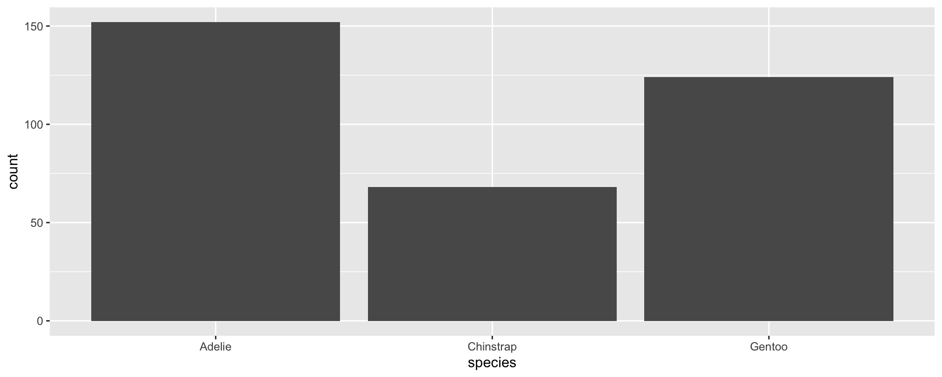
Changing the factor order: fct_infreq()
We may want to change the default factor order (alphabetical) and rearrange the order on the x axis. forcats:: gives us lots of options for rearranging our factors without having to manually list out all of the levels.
fct_infreq() allows us to sort by occurrence:

Changing the factor order: fct_rev()
fct_rev() flips the order in reverse
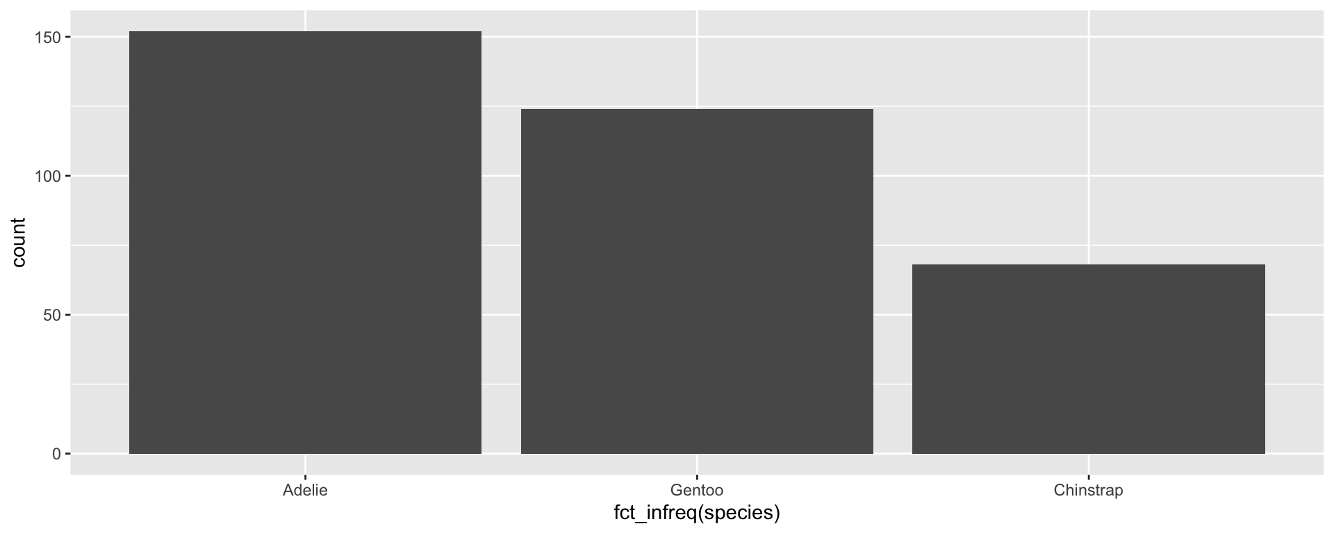

If you’re doing a lot of different analyses and visualization, you may want to change the factor order quite often.
Consider using these functions locally within your code so that you’re not actually changing the underlying dataset and future analyses.
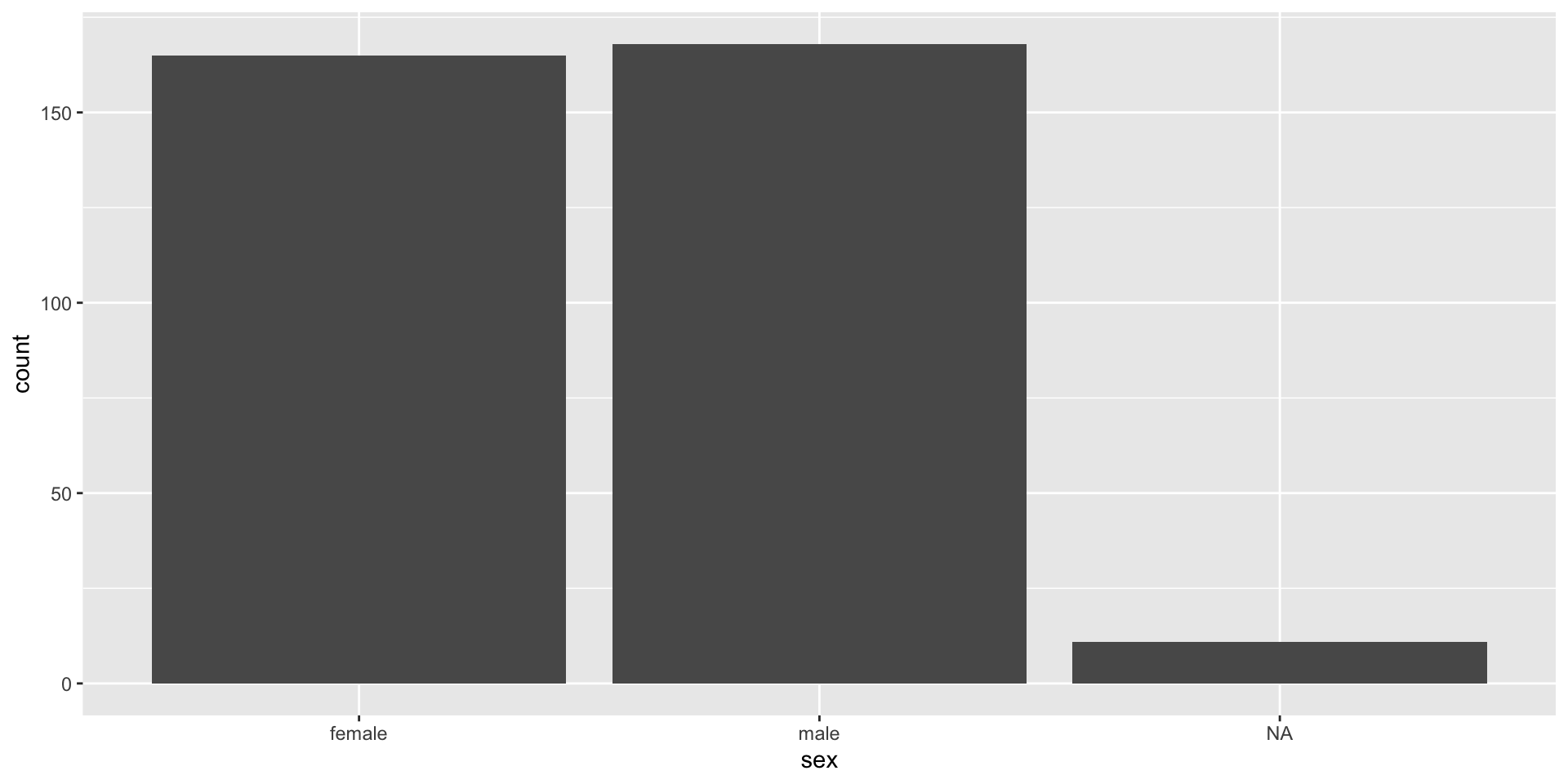
Factor rules: Missingness
Factors have a specific set of rules for missing values
- Factors retain NAs, but do not return NAs as a level by default
- Helpfully, it doesn’t drop NAs from the analysis, just because it’s not a level
- NAs will always be last in the factor order
Factor rules: Missingness

Factor rules: Missingness
Empty groups + NAs in factors
Once levels are set, they will be retained and kept consistent between groups, even when there is nothing in the group
NAs are not considered their own group by default
- They are not dropped, but they aren’t considered a “level”
Empty groups + NAs in factors
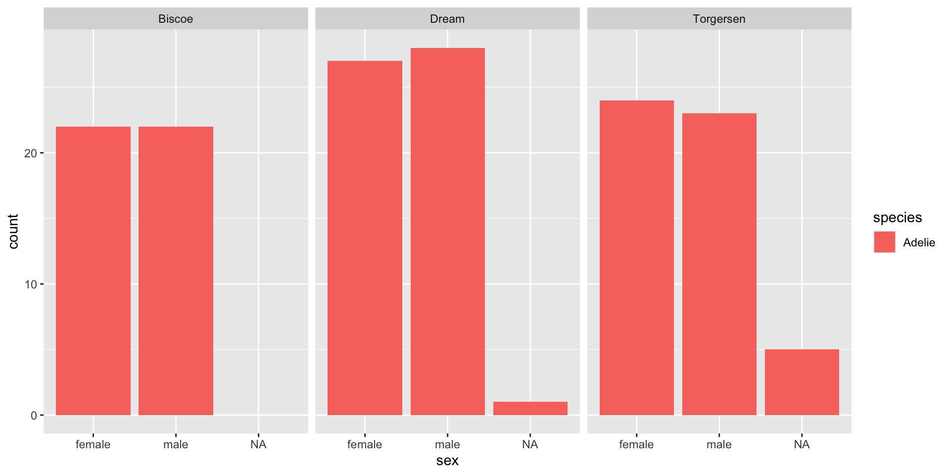
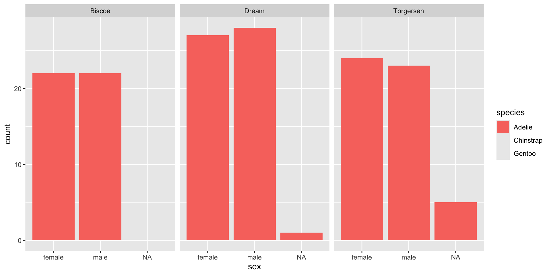
Let’s look at just the Adelie penguins.
Because species is a factor, the information about other species is retained, even when there is nothing in that category.
[1] Adelie
Levels: Adelie Chinstrap GentooEmpty groups + NAs in factors
Empty groups + NAs in factors
- Remember: NAs are not considered a factor level, so if we filter out the NAs, they will not be included in the legend even if we specify to keep all levels.
Example: NHANES
Let’s say we want to turn a continuous variable into categorical groups:
Age quartiles
Clinically relevant blood pressure categories
Creating age quartiles
   Min. 1st Qu.  Median    Mean 3rd Qu.    Max.
12.00 23.00 42.00 42.78 60.00 80.00 [1] "integer"Transforming age_quartiles into a factor
[1] "factor"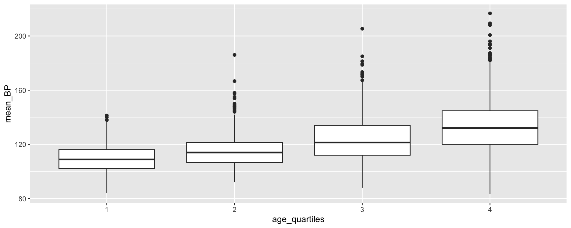
Transforming age_quartiles into a factor
What if we wanted the labels to convey more information?
[1] (23-42) (60-80) (12-23) (42-60)
Levels: (12-23) (23-42) (42-60) (60-80)
Transforming age_quartiles into a factor

Creating blood pressure categories
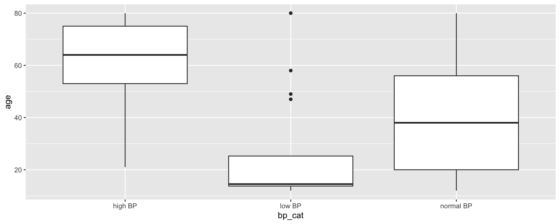
We also want to create clinically relevant categories of blood pressure:
Creating blood pressure categories
Because bp_cat is not a factor yet, R has plotted the variable in alphabetical order by default. There may be some situations where this is sufficient, but for ordinal data, the order of the data is important!
Transforming bp_cat into a factor
[1] normal BP high BP   low BP
Levels: high BP normal BP low BPWorking with Factors
The forcats:: package (short for “For Categorical”) is a helpful set of functions for working with factors.

Useful forcats:: functions
Check out the forcats:: cheatsheet for more info on how these functions work!
fct_drop()fct_relevel()fct_rev()fct_infreq()fct_inorder

⚠️ Caution: factors
Factors operate under a very strict set of rules. If you aren’t careful, you can accidentally create issues in your dataset
⚠️ Caution: factor → numeric
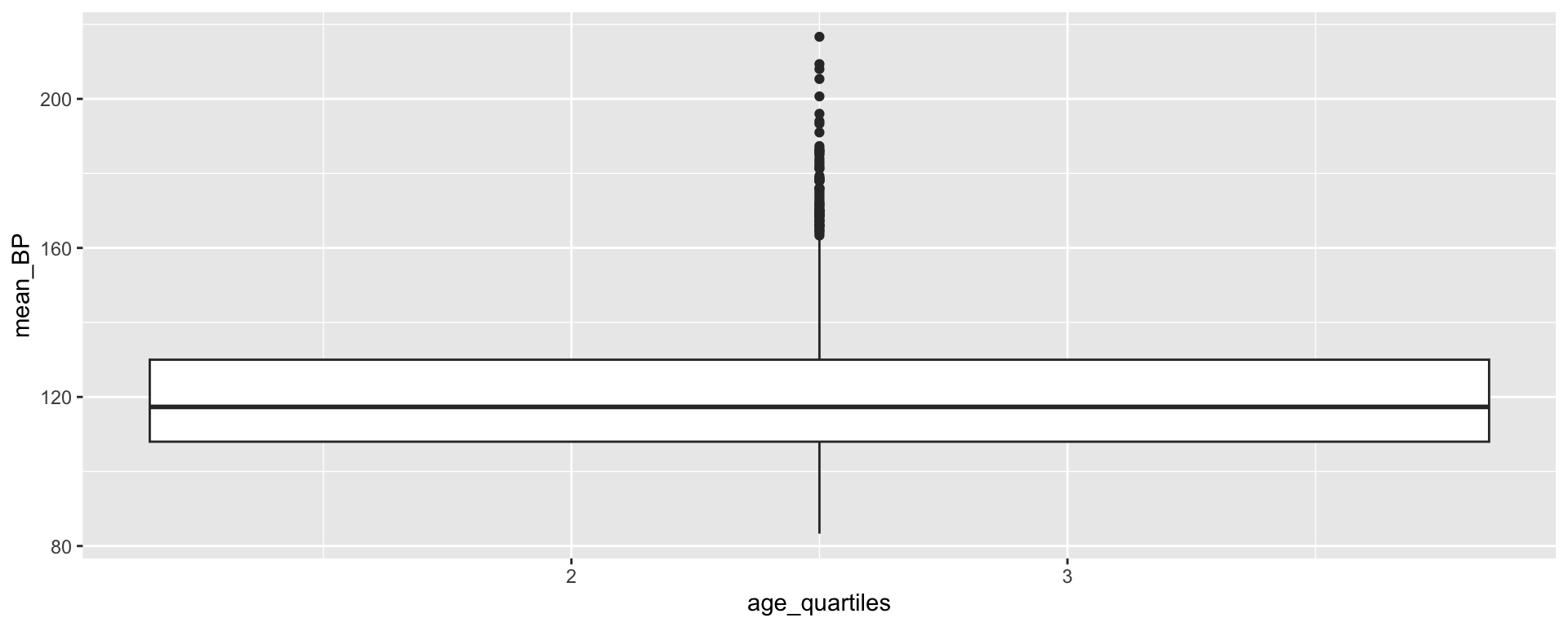
Let’s say we wanted to transform a “year” column from an integer to a factor to make a plot with a different boxplot for each year:
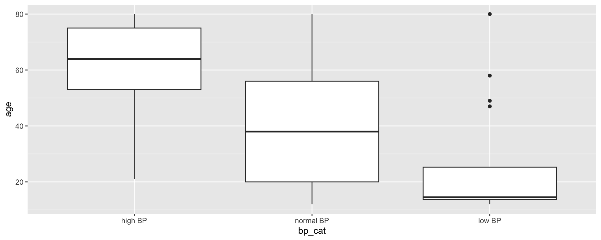
⚠️ Caution: factor → numeric
Later in your script, you decide you want to include year as a continuous variable, so you transform year into an integer.
[1] 1 2 3Oh no!
So what do you do?
- In some cases, you may want to set factors locally within a particular piece of your script, rather than globally.
- For example, you could run
as.factor()aroundyearwithin yourggplot().
⚠️ Caution: typos
If you don’t have exact matches when you assign factor levels and labels, you’re going to end up with a lot of NAs
penguins_sizes <- penguins %>%
  mutate(size_cat = case_when(bill_length_mm > mean(bill_length_mm, na.rm = T) &
                                bill_depth_mm > mean(bill_depth_mm, na.rm = T) &
                                flipper_length_mm > mean(flipper_length_mm, na.rm = T) ~ "big penguins",
                              bill_length_mm < mean(bill_length_mm, na.rm = T) &
                                bill_depth_mm < mean(bill_depth_mm, na.rm = T) &
                                flipper_length_mm < mean(flipper_length_mm, na.rm = T) ~ "small penguins",
                              TRUE ~ "average penguins"))

table(penguins_sizes$size_cat, useNA = "ifany")
average penguins     big penguins   small penguins
293 20 31 Date-Times
Working with dates
- What are some challenges you might anticipate working with dates?
Working with dates
Often, we need dates to function as both strings and numbers
As strings, we want to have a fair amount of control over how they are presented.
As numbers, we may want to add/subtract time, account for time zones, and present them at different scales.
Working with dates
There are lots of packages and functions that are helpful for working with dates. We’ll talk primarily about the lubridate:: package, but the goal today is to understand the components and rules of date-time objects so that you can apply these functions in your work.
Working with dates
There are 3 ways that we will work with date/time data:
dates
times
date-times
Working with dates 🤯😳
For the most part, we’re going to try to work with dates as Date objects, but you may see a date that defaults to POSIXct.
All computers store dates as numbers, typically as time (in seconds) since some origin. That’s all that POSIXct is – to be more specific, it is the time in seconds since 1970 in the UTC time zone (GMT).
From this point forward, all times will be presented in 24-hour time!!
Working with dates
To get an idea of how R works with dates, let’s ask for the current date/time:
Working with dates
But how do we actually work with this data? In practice, we might want to:
- Know how much time has elapsed between two samples
- Collapse daily measurements into monthly averages
- Check whether a measurement was taken in the morning or evening
- Know which day of the week a measurement was taken on
- Convert time zones
lubridate::
The lubridate:: package is a handy way of storing and processing date-time objects. lubridate:: categorizes date-time objects by the component of the date-time string they represent:
- year
- month
- day
- hour
- minute
- second

lubridate:: basics

Once you have a date-time object, you can use lubridate:: functions to extract and manipulate the different components.
lubridate:: basics

The function now() returns a date-time object, while today() returns just a date. lubridate:: also has functions that allow us to force the date into a date-time and the date-time into a date:
lubridate:: basics

With lubridate::, we can also work with dates as a whole, rather than their individual components. Let’s say we have a character string with the date, but we want R to transform it into a date-time object:
Time spans
There are three classes we can apply to our date-times so that we can work with them arithmetically 🧙️
- durations (measured in seconds)
- periods (measured in weeks/months)
- intervals (have a start and end point)
Time spans
Time spans
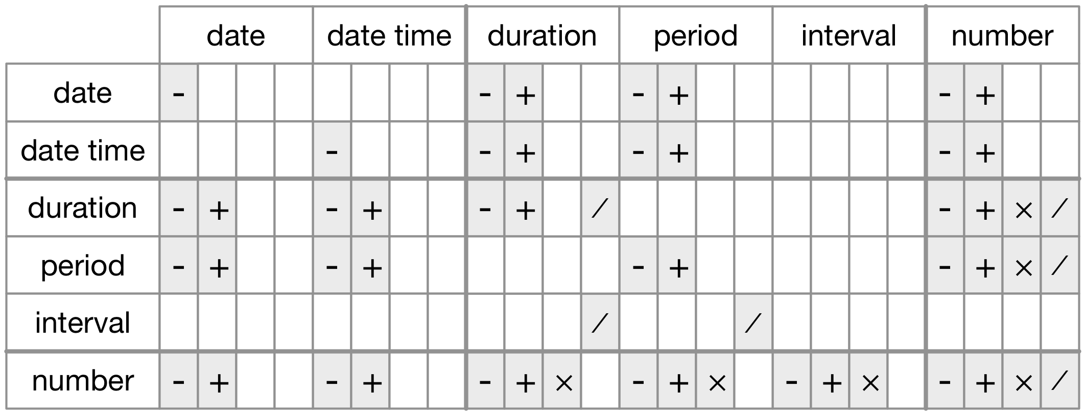
From R4DS Chapter 16: Dates and times
Supplemental date-time slides
Topics covered:
Durations vs Periods vs Intervals
WARNING: How to avoid time travel + other nuances
- Avoiding issues when collaborating
- Time is a construct: leap years + daylight savings time
Classroom CO_2 example
First day live coding demo example
Durations: Subtraction
We can use arithmetic operators with durations:
Time difference of 4 hours
Durations: Multiplication
What if we want to know the total amount of time you get to spend together? 😊
[1] "2026-01-12" "2026-01-13" "2026-01-14" "2026-01-15" "2026-01-16"
[6] "2026-01-20" "2026-01-21" "2026-01-22" "2026-01-23"Durations: Addition
How else might we calculate it?
class_meeting_times <- tibble(dates =  class_dates,
                              week = c(rep(1, 5), rep(2, 4)),
                              start_time = c(rep(hms("13:30:00"), 9)),
                              start_datetime = c(ymd_hms(paste(dates, start_time), tz = "EST")),
                              end_time = c(rep(hms("17:30:00"), 9)),
                              end_datetime = c(ymd_hms(paste(dates, end_time), tz = "EST")),
                              class_time_int = interval(start = start_datetime,
end = end_datetime))Periods
Since periods operate using “human” time, we can add to periods using functions like minutes(), hours(), days(), and weeks()
Intervals
Intervals can be created with the interval() function or with %--%. By default, intervals will be created in the date-time format you input.
[1] 2026-01-14 UTC--2026-01-23 UTC[1] 2026-01-14 UTC--2026-01-23 UTCWe can use %within% to check whether a date falls within our interval:
⚠️ Caution: Working with intervals, durations, and periods
⚠️ Caution: time is a construct 🫠
Leap years
Daylight savings
- durations measure consistent time in seconds
- periods work more like “human” time
Example: Classroom CO\(_2\)
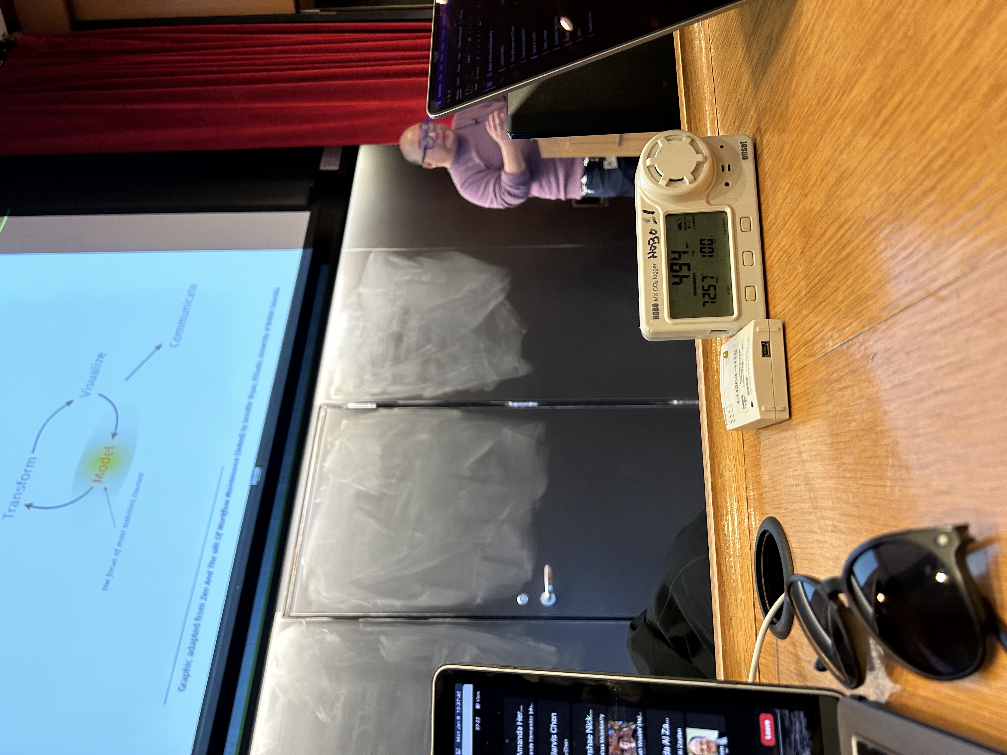
On the first day of ID529 in January 2023, Amanda set up an instrument to log indoor temperature, relative humidity, and CO\(_2\) in G2.
The logger (called a HOBO) was set to collect data at 1-second intervals ~15 minutes before class began and ~15 minutes after class ended.
The data were cleaned and are now “long”
Example: Classroom CO\(_2\)
jan23_meeting_times <- tibble(dates =  c(seq(ymd('2023-01-09'),ymd('2023-01-13'), by = 1),
                                        seq(ymd('2023-01-17'),ymd('2023-01-20'), by = 1)),
                             week = c(rep(1, 5), rep(2, 4)),
                             start_time = c(rep(hms("13:30:00"), 9)),
                             start_datetime = c(ymd_hms(paste(dates, start_time), tz = "EST")),
                             end_time = c(rep(hms("17:30:00"), 9)),
                             end_datetime = c(ymd_hms(paste(dates, end_time), tz = "EST")),
                             class_time_int = interval(start = start_datetime,
                                                       end = end_datetime))

hobo_g2_dt <- hobo_g2 %>%
  mutate(metric = factor(metric, levels = c("co2_ppm", "temp_f", "rh_percent"),
                         labels = c("CO2 (ppm)", "Temperature (F)", "Relative Humidity (%)")),
         date_time = force_tz(as_datetime(date_time), tz = "EST"),
         time = hms::as_hms(date_time),
         date = as_date(date_time),
         hour = hour(date_time),
         minute = minute(date_time),
         second = second(date_time))

glimpse(hobo_g2_dt)
Rows: 51,303
Columns: 8
$ date_time <dttm> 2023-01-09 13:15:00, 2023-01-09 13:15:00, 2023-01-09 13:15:…
$ metric <fct> Temperature (F), Relative Humidity (%), Temperature (F), Rel…
$ result <dbl> 71.834, 34.128, 71.834, 33.995, 71.834, 33.929, 71.834, 33.7…
$ time <time> 13:15:00, 13:15:00, 13:15:01, 13:15:01, 13:15:02, 13:15:02,…
$ date <date> 2023-01-09, 2023-01-09, 2023-01-09, 2023-01-09, 2023-01-09,…
$ hour <int> 13, 13, 13, 13, 13, 13, 13, 13, 13, 13, 13, 13, 13, 13, 13, …
$ minute <int> 15, 15, 15, 15, 15, 15, 15, 15, 15, 15, 15, 15, 15, 15, 15, …
$ second <dbl> 0, 0, 1, 1, 2, 2, 3, 3, 4, 4, 5, 5, 6, 6, 7, 7, 8, 8, 9, 9, …Example: Classroom CO\(_2\)
ggplot(hobo_g2_dt, aes(x = date_time, y = result))  +
  geom_line() +
  facet_wrap(~metric, scales = "free_y", ncol = 1) +
  scale_x_datetime(breaks = scales::date_breaks("30 mins"), date_labels = "%H:%M") +
  xlab("Time") +
  ylab("") +
  ggtitle(paste0("Indoor conditions in G2 (", unique(hobo_g2_dt$date), ")"))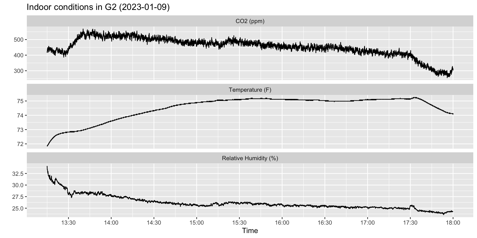
Example: Classroom CO\(_2\)
Often, we have really granular data that we want to report in some aggregate form. This data is measured in 1-second intervals, but let’s say we wanted to calculate a 1-minute average or an hourly average.
Because we separated date_time into it’s various components, we can now use group_by() and summarize() to calculate averages.
hobo_g2_1min <- hobo_g2_dt %>%
  group_by(metric, date, hour, minute) %>%
  summarize(avg_1min = mean(result)) %>%
  mutate(date_time = ymd_hm(paste0(date, " ", hour, ":", minute), tz = "EST"))

hobo_g2_1hr <- hobo_g2_dt %>%
  group_by(metric, date, hour) %>%
  summarize(avg_1hr = mean(result)) %>%
  mutate(date_time = ymd_h(paste0(date, hour), tz = "EST"))
Example: Classroom CO\(_2\)

Example: Classroom CO\(_2\)
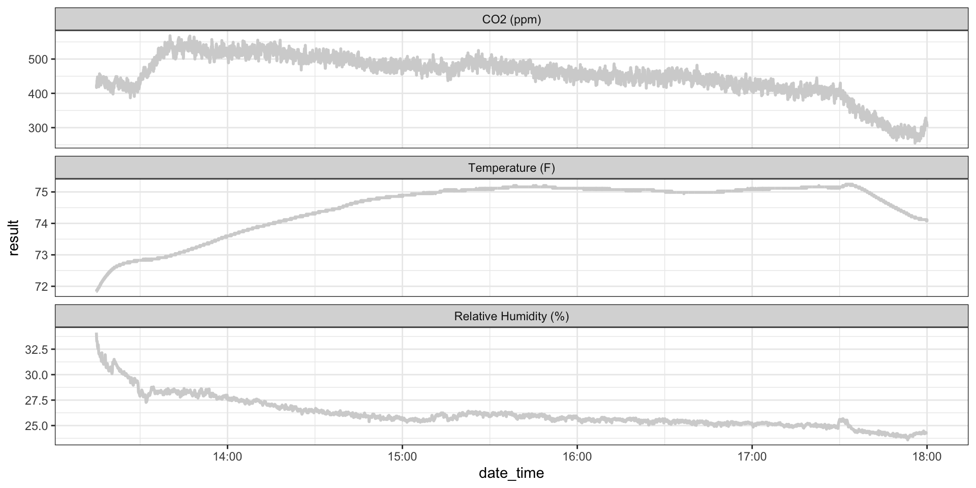
Example: Classroom CO\(_2\)
ggplot(hobo_g2_dt, aes(x = date_time, y = result))  +
  geom_line(color = "lightgrey", size = 1) +
  geom_line(hobo_g2_1min, mapping = aes(x = date_time, y = avg_1min), color = "slateblue3") +
  geom_line(hobo_g2_1hr, mapping = aes(x = date_time, y = avg_1hr), color = "paleturquoise2", alpha = 0.7) +
  facet_wrap(~metric, scales = "free_y", ncol = 1) +
  theme_bw()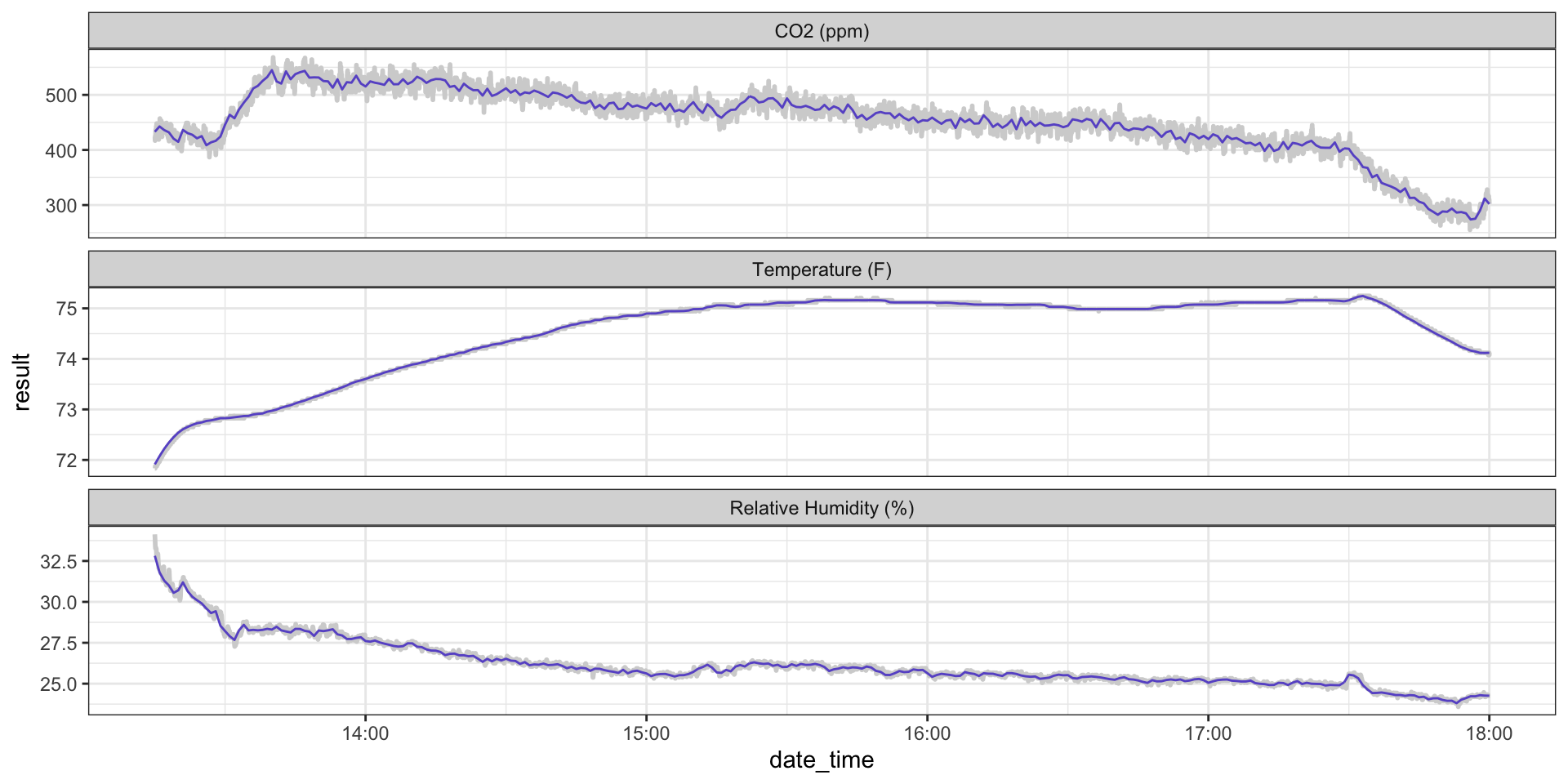
Example: Classroom CO\(_2\)
Another thing we might be interested in is whether a measurement occurred during a specific interval, for example, during class time.
We can use %within%, which works similarly to %in% but for date-times.
Example: Classroom CO\(_2\)
ggplot(hobo_g2_dt)  +
  geom_line(aes(x = date_time, y = result), color = "lightgrey", size = 1) +
  geom_line(hobo_g2_1min, mapping = aes(x = date_time, y = avg_1min), color = "slateblue3") +
  geom_line(hobo_g2_1hr, mapping = aes(x = date_time, y = avg_1hr), color = "paleturquoise2") +
  geom_rect(data = jan23_meeting_times %>%
              filter(dates %in% hobo_g2_dt$date),
              mapping = aes(xmin = start_datetime,
                            xmax = end_datetime,
                            ymin = 0, ymax = Inf),
              alpha = 0.2, fill = "lightpink") +
  facet_wrap(~metric, scales = "free_y", ncol = 1) +
  theme_bw()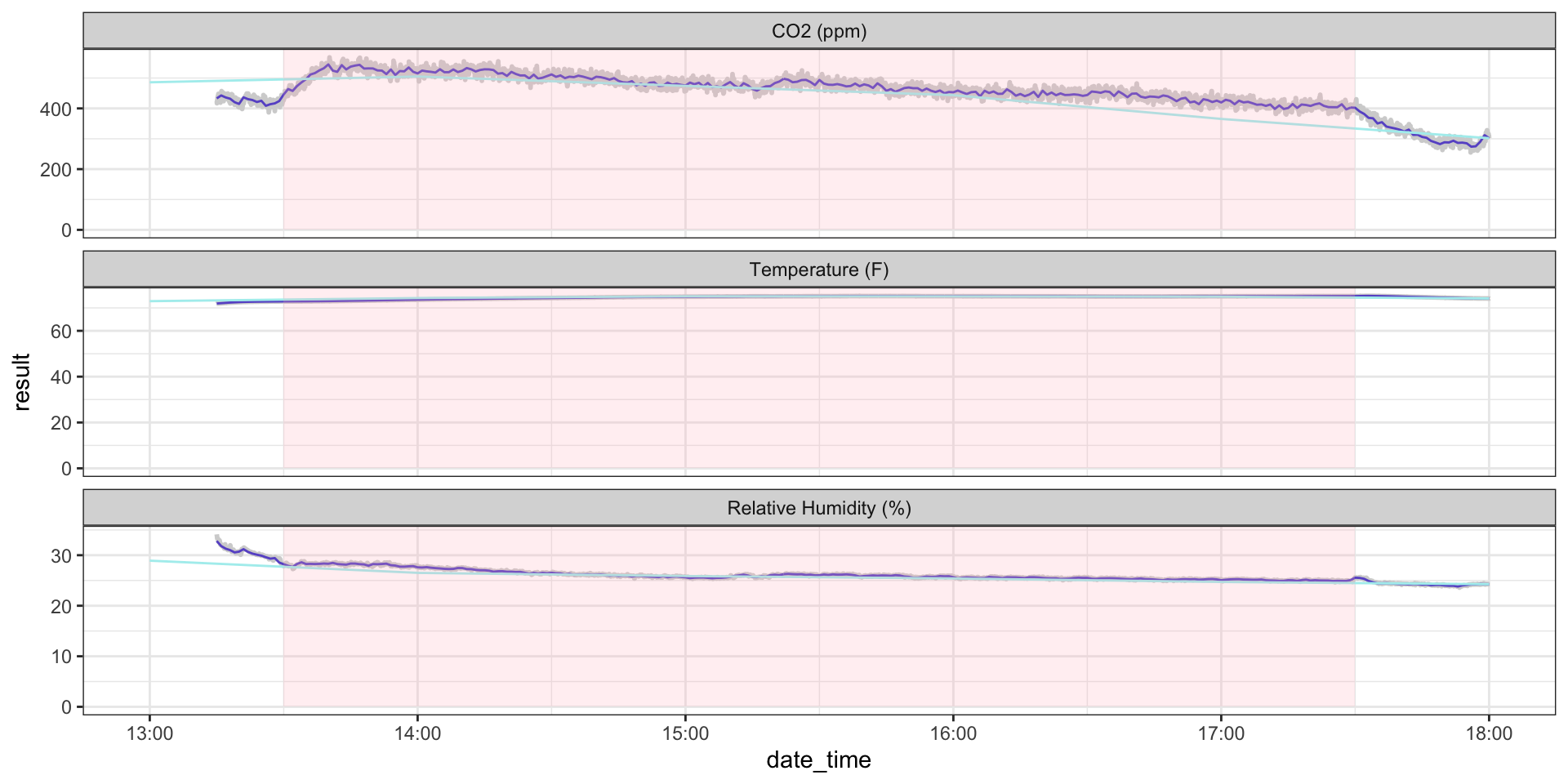
Example: COVID data
If you can remember back to the demo on the first day, Christian demonstrated an application of factors and date-times into his workflow
covid <- list(
  readr::read_csv("us-counties-2020.csv"),
  readr::read_csv("us-counties-2021.csv"),
  readr::read_csv("us-counties-2022.csv")
)

# convert to 1 data frame
covid <- bind_rows(covid)


# cleaning covid data -----------------------------------------------------------

# create year_month variable
covid$year_month <- paste0(lubridate::year(covid$date), "-",
                           lubridate::month(covid$date))

# aggregate/summarize by year and month by county
covid <- covid |>
  group_by(geoid, county, state, year_month) |>
  summarize(deaths_avg_per_100k = mean(deaths_avg_per_100k, na.rm=TRUE))

# cast year_month to a factor
year_month_levels <- paste0(rep(2020:2023, each = 12), "-", rep(1:12, 4))
covid$year_month <- factor(covid$year_month, levels = year_month_levels)
Example: COVID data
ggplot(
  covid_by_poverty_level |> filter(! is.na(poverty_cut)),
  aes(x = year_month,
      y = deaths_avg_per_100k,
      color = poverty_cut,
      group = poverty_cut)) +
  geom_line() +
  scale_color_brewer(palette = 'RdBu', direction = -1) +
  xlab("Date") +
  ylab("COVID-19 Mortality per 100k (monthly observations)") +
  ggtitle("Monthly County COVID-19 Mortality Estimates by Poverty Level in the US") +
  theme(axis.text.x = element_text(angle = 75, hjust = 1))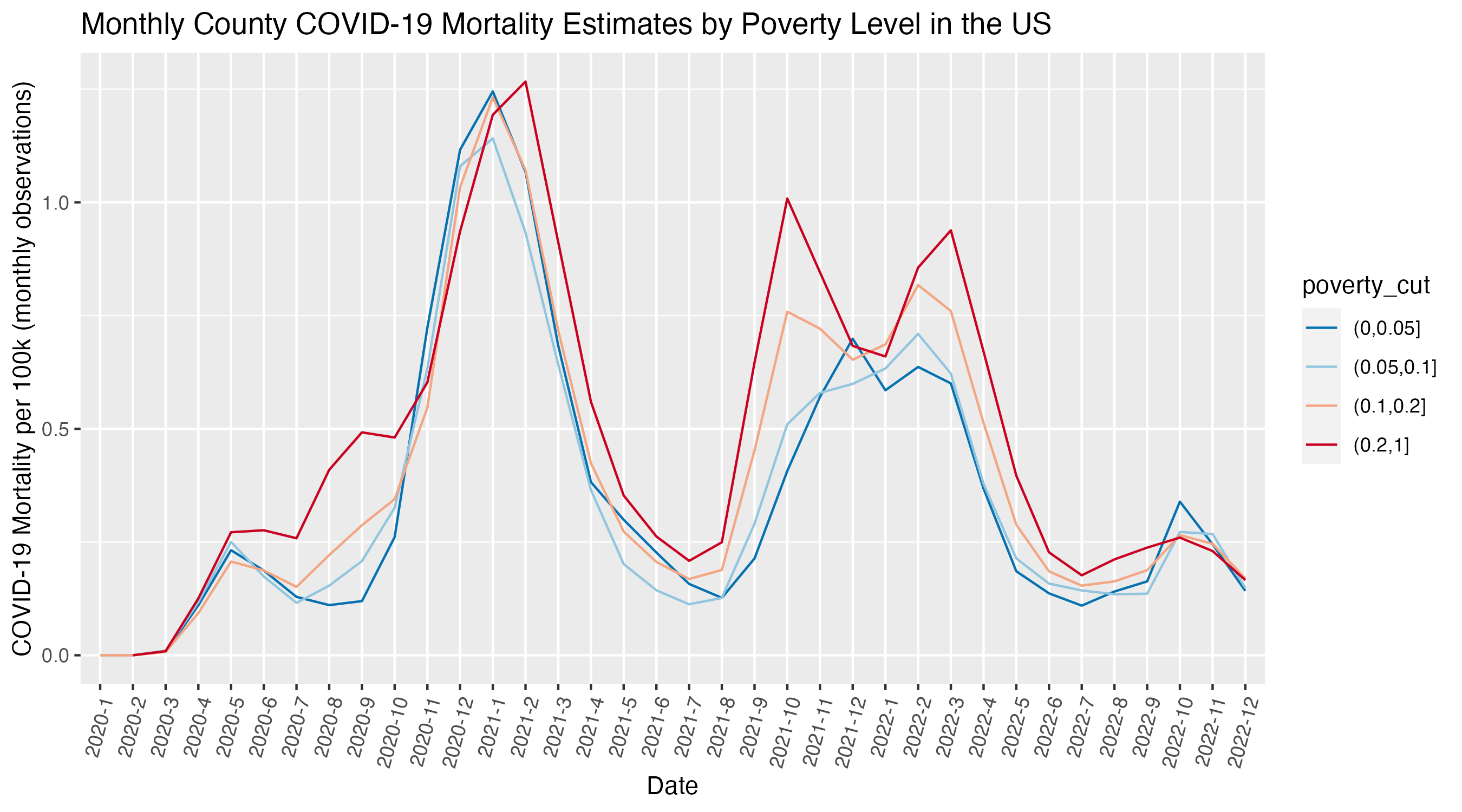
Key takeaways
Knowing how to manipulate factors and date-times can save you a ton of headache – you’ll have a lot more control over your data which can help with cleaning, analysis, and visualization!
forcats::andlubridate::give you a lot of the functionality you might needhms::is another package for working with times (stores time as seconds since 00:00:00, so you can easily convert between numeric and hms)
Factors and date-times can be tricky
Double check things are working as you expect along the way!!
If you can’t figure out why something isn’t working, take a break, and revisit it with fresh eyes.
There’s lots of documentation out there! The cheatsheets are great, as is The Epidemiologist R Handbook (https://epirhandbook.com/en/working-with-dates.html#working-with-dates-1)
